Alan Tarica, Pratik Tambe, Tom Crone and I have been pulling our hair out for a couple of years, trying to use cameras and software to measure the ‘figure’ of the telescope mirrors that we and others produce in our telescope-making class.

There has been progress, and there has been frustration.

I think we finally succeeded!

Some of the difficulties have been described in previous posts. In brief, we want our mirrors to be really, really close to a perfect paraboloid. There are many ways of doing those measurements and seeing whether one is close enough, but none of those methods are easy!

(By the way, one needs the entire mirror to be within one-tenth of a wave-length of green light of that ideal paraboloid! That’s extremely tiny, and equivalent to the thickness of a pencil over a ten-mile diameter!)

I think I can finally report a victory. My evidence is this graph that I made just now, using data that Alan and I gathered last night with our setup, which consists of a surveillance camera coupled to an old 35mm SLR film camera lens, which is mounted on a linear actuator screw connected to a stepper motor controlled by an Arduino and a Python app developed by Pratik.

Something seemed to be always a bit — or a lot — ‘off’.

Until today, when I converted everything to millimeters and used the criterion set out by Adrien Millies-Lacroix in an article he wrote in Sky & Telescope back in 1976.

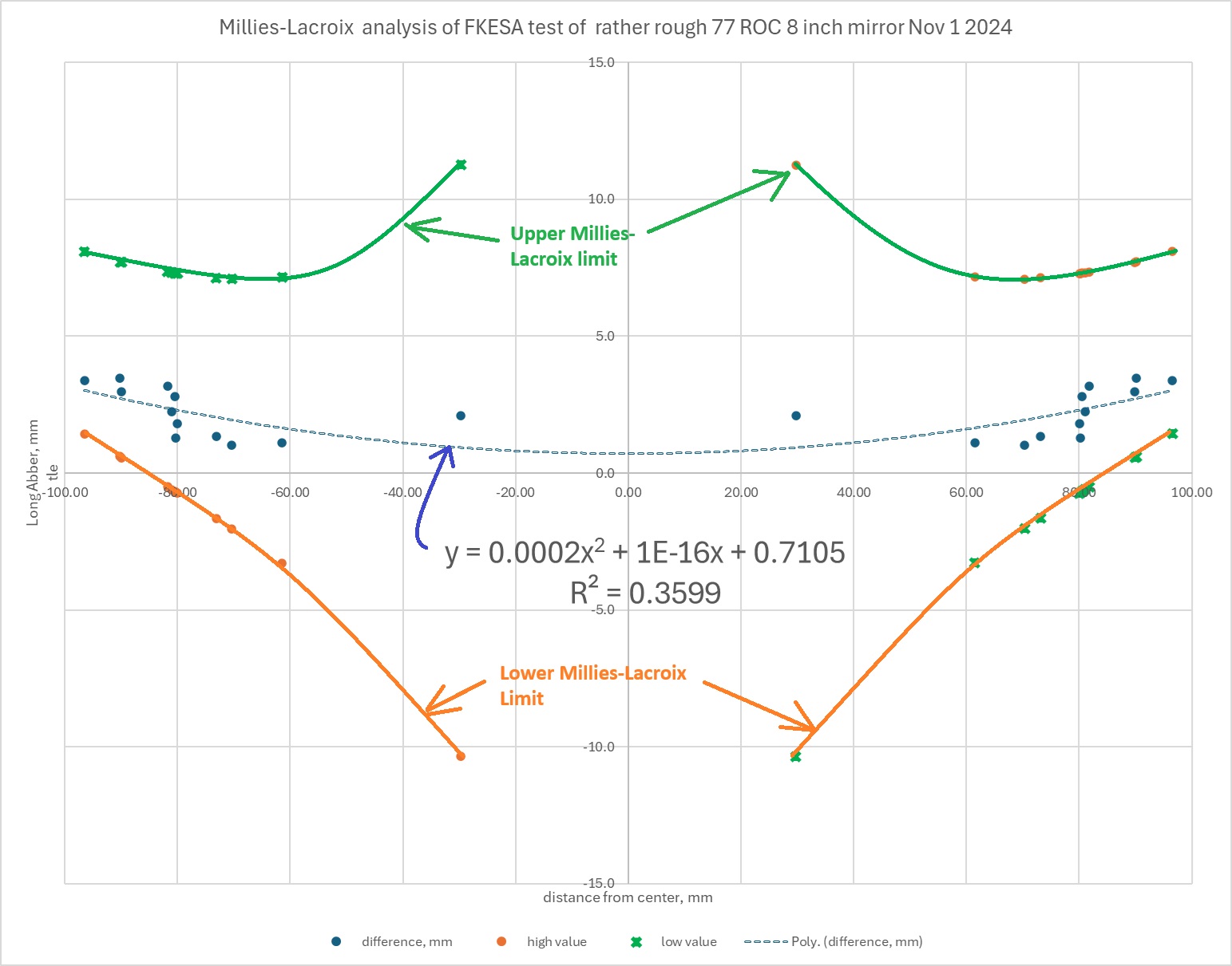
The blue dots just above the x-axis are the measurements for this one particular mirror with a diameter of 8″ and a radius of curvature of 77 inches.

The dotted blue curve in the middle of the image is the best-fit parabola for those dots. Notice that the R-squared value (variance) for that curve is not great: 0.3599.

But that variance isn’t important. What is important is the green and orange blobs and curves above and below the blue ones.

The green and orange curves are the upper and lower allowable limits for the measurements of this particular mirror, using the

Clearly, the blue dots are all well within the green and orange curves.

Which means that this mirror is sufficiently parabolized.

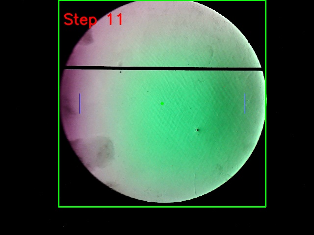
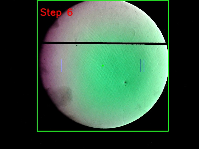
The fact that the blue dots don’t fit the dotted line perfectly, and behave pretty oddly at positive or negative 80 millimeters, both agree with the fact that we can see on the photos that the surface of this mirror is rather rough, as you can see in the images below. Note also that the image labeled ‘Step 6’ found not one, but two null zones on the right, indicated by two vertical blue lines.

So, finally, we have an algorithm that gives good measurements! What I still want to do is to automate all the spreadsheet calculations that I just did today. Perhaps we can upload them to something like FigureXP by Dave Rowe and James Lerch.

Thanks very much to all those who have helped, whom I should look up and name here.

Caveat: This method can give really ridiculous measurements close to the center and close to the edge.

PS: if anybody wants the raw data, just email me at gfbrandenburg at gmail dot com.