This time I attempted to detect a different transit of another star using two different setups on the grounds of Hopewell Observatory in northern Virginia.
A Canon 6D DSLR mounted on a big, heavy 14-inch Schmidt-Cassegrain telescope on a very sturdy AP1600GTO equatorial mount
An alt-az Seestar S50 all-in-one astro camera
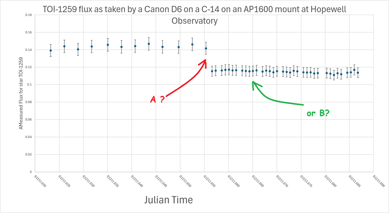
Can you spot where the exoplanet TOI-1259-b dimmed the light from its host star?
(Hint: this is a trick question!)
Here are the graphs I made from the data I collected:
Was it at A? Or did it happen at B? (Trick question!)
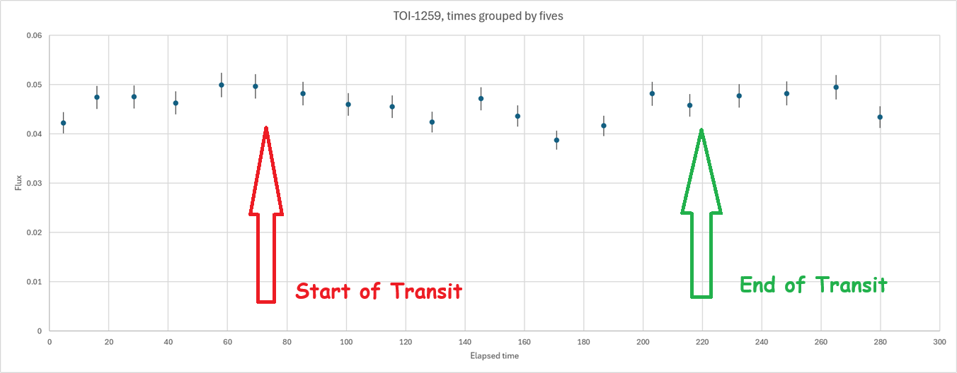
And this graph is what I got from my SeestarS50:
Psst:
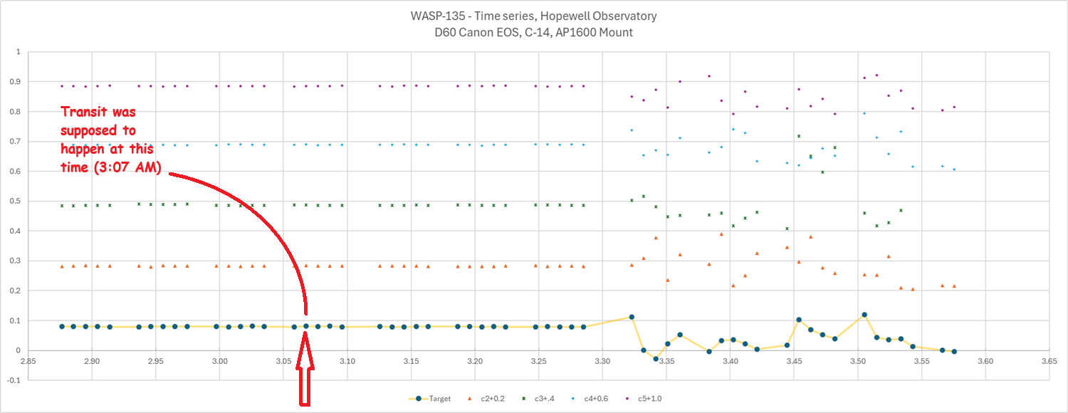
Point A in the first graph was when I reduced the exposure time on the camera from 2 minutes to 30 seconds. That caused all of the fluxes to decrease, because cutting the time by 4 reduces the number of photons captured. Arrow B points to where the transit was supposed to happen, with a 2.7% decrease in brightness.
Do you see it?
Me neither.
In the second graph, done by the Seestar at the same location on the same night, smoothed as much as I can by averaging successive images, I again don’t see much evidence of a 2.7% dip in total flux.
Conclusion: chasing exoplanet transits looks like it could be easy, but it’s not.
===============
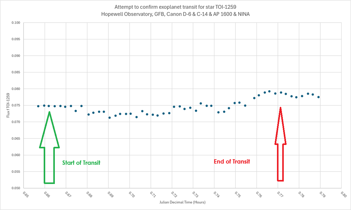
This graph here is no better.
And here is where I extracted just the two green channels:
No, I am not at all convinced that my measurements captured anything.
Do you see a transit in this data? I would say, “Maybe”.
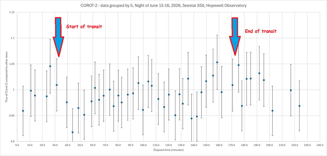
Since the Seestar has quite a bit of error, caused in part by its Bayer array of green, red, and blue pixels, I grouped my original measurements (processed in AstroImageJ) in groups of 5, using Excel to do so.
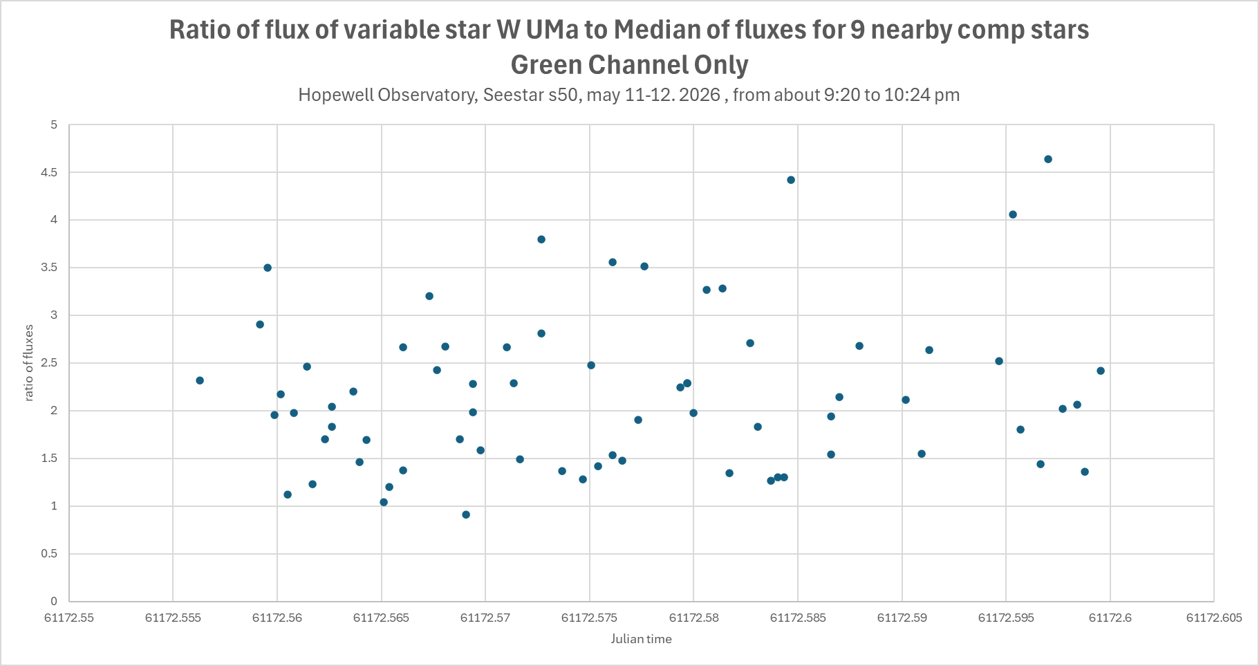
Latest results on a known variable star, W Ursae Majoris with my Seestar S50 during a very nice night: complete garbage. The graph below shows the flux of my star, WUMa, compared to the median of 9 comparison stars in the same frame, chosen by AstroImageJ.
As you can see, there is no real pattern.
If this data were real, then this star would be changing its brightness by a factor of three or for in less than a minute, with no discernable pattern. While a candle flame will flicker like that, it is simply not possible for something as large as a star to vary as quickly as that. In fact, this star is actually a contact-binary (double star) with a rotational period of about 8 hours. Even with the noise, I see no sign of a trend over these two hours.
The weather was very good, there was very little light pollution, and this star was quite high up in the sky the entire time, and none of the stars were saturated. But this data is just so, so noisy.
(I used ASTAP and AstroImageJ to do the plate solving and comparison of brightnesses. AIJ is an absolutely amazing program that automates so much of the tedium of this sort of process. For this graph, I had AIJ extract the green channel from the GRGB Bayer pattern, hoping that eliminating the blue channel would reduce atmospheric problems, but no luck so far. Combining all channels was no better.)
Other people claim success, but so far I’m zero for 12 in detecting exoplanet transits, and only 1 out of a dozen or so variable star measurements. Not sure what I am doing wrong or how I can reduce the errors. Yes, it’s true that this is only 2 hours out of an 8-hour period, but this data does not make any sense!
As you probably have guessed, detecting exoplanets is not easy.
So far I am about zero detections for 12 attempts.
My equipment has been a Seestar S50, and either a ZWO CMOS camera on an Explore Scientific 5″ f/7 triplet refractor, and a Canon 6D DSLR affixed to a venerable C-14 mounted on an Astrophysics 1600 GTO mount.
The Seestar is able to detect brightness changes in other variable stars like RRLyrae, but so far the small changes in flux from exoplanet transits gets drowned in the noise. The DSLR on the C-14 has much less noise, but I still haven’t seen any clear and obvious signs of a transit.
Here are graphs from my latest attempt at detecting WASP-135-b. In the first one, I plotted the fluxes of that star against four of the comparison stars. I added a fixed number to the fluxes of the other stars so you could see trends more clearly. Shortly after 3:30 AM, measurements became very strange for every single star. I was asleep at that time. I’m guessing that there were clouds. Do you see any noticeable dip in brightness of the target star at 3:07? I sure don’t.
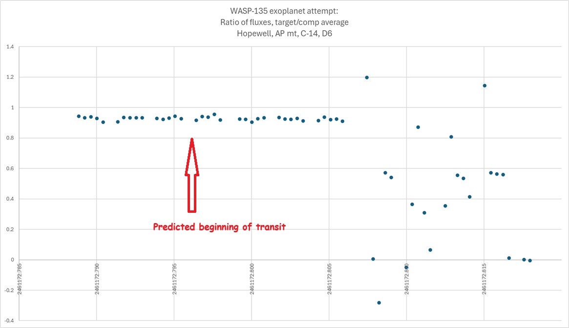
In the second graph, I asked Excel to take the average of the fluxes of several of the comparison stars, and then divide the flux from WASP-135 by that average. Again, I see no dip at the appropriate time (Julian Day).
I used NINA to program my cameras and the Hopewell Observatory’s AP mount to take these images. I used ASTAP and AstroimageJ to load all of the images from my various cameras, figure out exactly where the cameras were pointing (aka plate solving), find a bunch of comparison stars, and then measure the fluxes of each of those stars, on each and every single 30-second frame. That set of software — all free!!!– has made all of this work much easier. Thank you to all the incredibly smart and generous people who wrote, and then made freely available, all those complicated computer programs!
I will try TOI-1811 tonight, with some different settings.
Most (but not all) of the variable stars I tried over the past month or so were simply too bright for this sensor. The target stars were saturated (ie some of the pixels’ electron wells simply overflowed) despite using the shortest available exposure, adding the light pollution filter and refocusing. Seestar won’t let your change the ISO nor open the shutter for less than 10 seconds.
I did get some believable light curves on BE Lyncis (aka HD67390)and U Cephii (aka HD 5679). I attack some graphs I made.
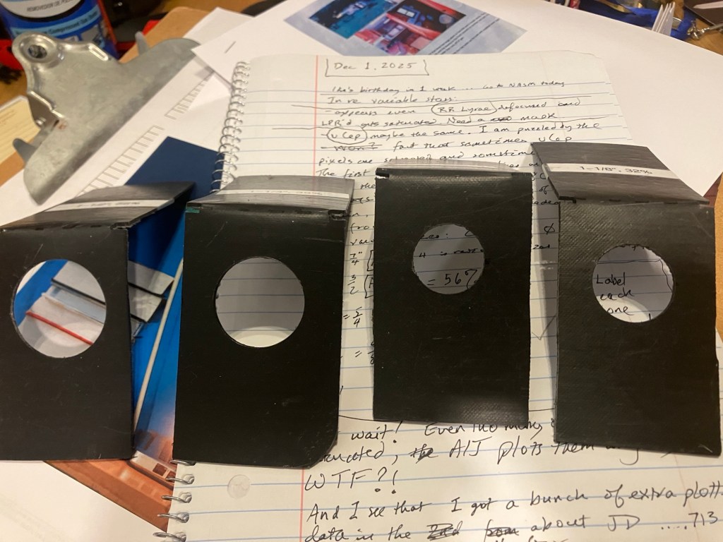
I used some black plastic I had,and my set of Forster bits, to make holes of sizes 1”, 1-1/8”, 1-1/4”, and 1-1/2”, in case I want to try brighter variable stars again like RR Lyrae.
I very impressed that Seestar absolutely nails the locations of every single one of these targets! I’m also pleased that AstroImageJ allows quick and easy plate-solving!
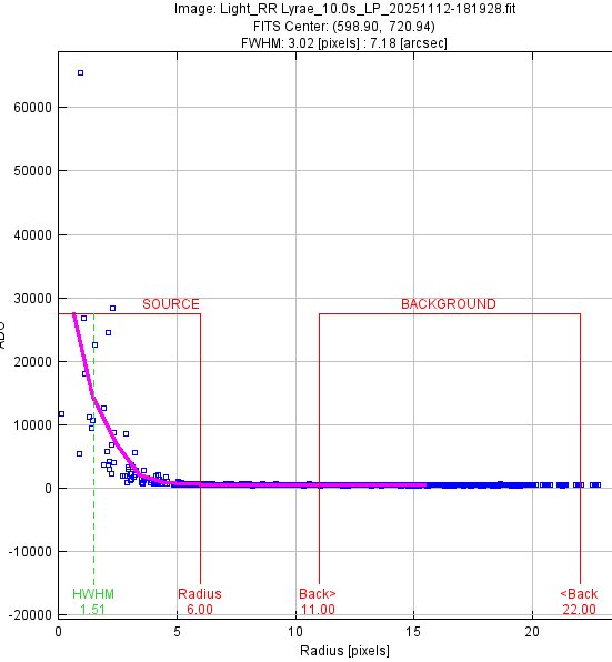
This graph gives me confidence that defocusing will solve my overflow problem. It’s a profile of the number of photons/electrons captured (vertical axis) versus the distance from what I thought was the exact center of the star RR Lyrae aka HD 182989.
(It is amazing how fast the computer works this out! I’m used to my middle school or high school students working things out like this by hand at first — it’s a very slow and tedious process! Let us give a tip of the hat to Williamina Fleming, who was the first person to notice and record that RR Lyrae was a variable star. She did so by examining glass plates on which were little dark spots made by stars’ light striking particles of suspended silver nitrate, without a blink comparator! Wow!)
Notice that there is one
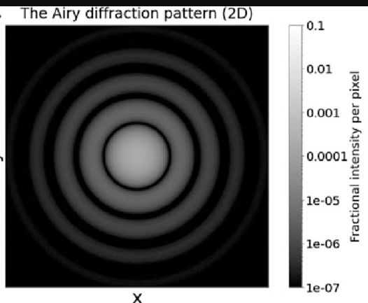
If I defocus the camera a bit, that saturated value would get spread out over an airy disk that might look like this:
We’ve all been brainwashed by years of Star Wars, Star Trek, Marvel Universe, Avatar, etc, to think that space should be teeming with intelligent civilizations, most of them vaguely like ourselves, working with and against each other to carve up the galaxy. As a result, it’s easy to overlook the huge assumptions embedded in your question.
Habitable worlds exist. Do they? It seems overwhelmingly likely, given that there are probably a trillion planets in the Milky Way alone, but for now we don’t know. Perhaps there are many near-miss planets like Venus and Mars, but extremely few true Earth analogs. For instance, life might require a particular rock/ice ratio, a large moon, and a specific style of plate tectonics. That level of specificity seems unlikely to me, but that’s just my random opinion. Until we find another planet with truly Earthlike conditions, we cannot say for sure that this is true.
Alien life exists. Does it? Honestly, we have no idea. There are many strong arguments suggesting that the fundamental biochemistry of self-replication is practically inevitable given the right conditions. But we don’t know how common those conditions are (see above), and even then we don’t know if there is some extremely low-probability gap that hinders the emergence of even simple microbial life.
Intelligent life exists. Does it? This one is a complete unknown. Keep in mind that there was no intelligent, self-aware life on Earth for 99.999% of its existence. Maybe the emergence of intelligence here was a rare fluke, unlikely to be reproduced anywhere else. Rat-level intelligence seems to have existed for at least 200 million years without any indication that higher level intelligence would confer a big evolutionary advantage. (There are all kinds of speculations about why intelligent life could not emerge until now on Earth, but these are just-so stories, trying to paint an explanation on top of a truth that we already know.)
Intelligent species want to “colonize” the galaxy. Do they? Life does have a tendency to explore every available ecological niche, and humans sure do like to spread out. From our example of one Earth, it seems likely that this is a general tendency of life everywhere, but we are doing an awful lot of extrapolating here. Maybe other types of intelligence have other motivations that have nothing to do with expansion.
Intelligent species become technological species. Do they? It’s certainly true for humans, but dolphins have a high level of intelligence and they are not trying to build spaceships. Crows, chimps, and bonobos are also capable of simple tool use, but they don’t appear to have experienced any evolutionary pressure to become true technological species.
Technological species can travel a significant fraction of the speed of light. (I assume you mean something like more than 1% of light speed.) Can they? Extrapolating from human technology, that seems extremely likely. Then again, the fastest spacecraft we have ever built would take about 300,000 years to reach the next star. Nobody is going to be colonizing the galaxy at that rate. You have to accept that speculative but unproven technologies are both feasible and practical for more advanced technological civilizations. Maybe intelligent life is out there, but in isolated pockets.
Intelligent, technological, space-faring species survive for a long time. Do they? Oh boy, we have no idea at all if this is true. Earth is 4.5 billion years old. Life has been around 4 billion years. Land species have been around 400 million years. Rat-level intelligence has maybe been around 200 million years. Our species has been around for about 100 thousand years. We have been capable of spaceflight for less than 100 years. It may seem inconceivable that humans could go extinct—but even if we last another 100,000 years, that may not be nearly enough time to spread across the galaxy, even if we develop the means to do it and maintain the will to do it. If intelligent species typically last less than 100,000 years, thousands of them could have come and gone in our galaxy without us ever knowing.
So there’s not one answer, but a whole set of overlapping possible answers why we don’t see evidence of any alien civilizations around us. And that doesn’t even consider more exotic possibilities, such as the idea that they might be here but just undetectable to us or deliberately hidden from our primitive eyes.
Alan Tarica, Pratik Tambe, Tom Crone and I have been pulling our hair out for a couple of years, trying to use cameras and software to measure the ‘figure’ of the telescope mirrors that we and others produce in our telescope-making class.
There has been progress, and there has been frustration.
I think we finally succeeded!
Some of the difficulties have been described in previous posts. In brief, we want our mirrors to be really, really close to a perfect paraboloid. There are many ways of doing those measurements and seeing whether one is close enough, but none of those methods are easy!
(By the way, one needs the entire mirror to be within one-tenth of a wave-length of green light of that ideal paraboloid! That’s extremely tiny, and equivalent to the thickness of a pencil over a ten-mile diameter!)
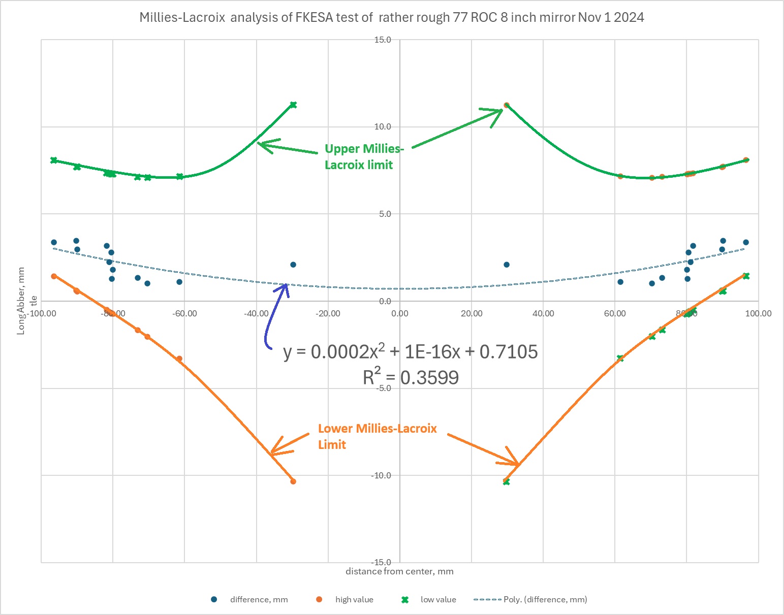
I think I can finally report a victory. My evidence is this graph that I made just now, using data that Alan and I gathered last night with our setup, which consists of a surveillance camera coupled to an old 35mm SLR film camera lens, which is mounted on a linear actuator screw connected to a stepper motor controlled by an Arduino and a Python app developed by Pratik.
Something seemed to be always a bit — or a lot — ‘off’.
The blue dots just above the x-axis are the measurements for this one particular mirror with a diameter of 8″ and a radius of curvature of 77 inches.
The dotted blue curve in the middle of the image is the best-fit parabola for those dots. Notice that the R-squared value (variance) for that curve is not great: 0.3599.
But that variance isn’t important. What is important is the green and orange blobs and curves above and below the blue ones.
The green and orange curves are the upper and lower allowable limits for the measurements of this particular mirror, using the
Clearly, the blue dots are all well within the green and orange curves.
Which means that this mirror is sufficiently parabolized.
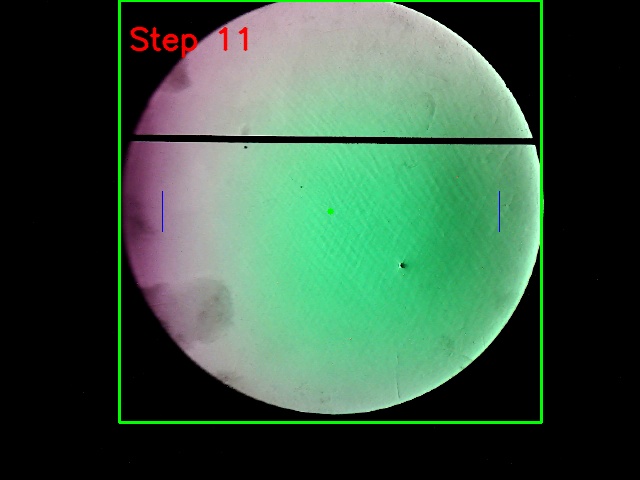
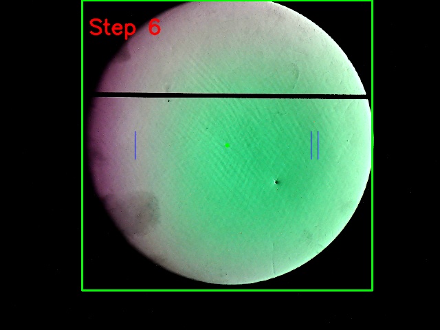
The fact that the blue dots don’t fit the dotted line perfectly, and behave pretty oddly at positive or negative 80 millimeters, both agree with the fact that we can see on the photos that the surface of this mirror is rather rough, as you can see in the images below. Note also that the image labeled ‘Step 6’ found not one, but two null zones on the right, indicated by two vertical blue lines.
So, finally, we have an algorithm that gives good measurements! What I still want to do is to automate all the spreadsheet calculations that I just did today. Perhaps we can upload them to something like FigureXP by Dave Rowe and James Lerch.
Thanks very much to all those who have helped, whom I should look up and name here.
Caveat: This method can give really ridiculous measurements close to the center and close to the edge.
PS: if anybody wants the raw data, just email me at gfbrandenburg at gmail dot com.
There is a pretty well-known paradox which goes something like this:
You hear that the Smith and Jones families each have two children.
You are told that the older Smith child is a girl, and that at least one of the Jones children is a girl.
Assuming that boys and girls are equally likely to be born (I know this is not quite true, but let’s pretend) in any given pregnancy, what are the chances that the Smiths have two girls? How about the Joneses?
Most people would say that those probabilities are equal: 50% in both cases.
But they are not. In fact, it is much less likely that the Joneses have two daughters!
Here is why:
In any family with two children, there is an older sibling and a younger one.
In the Smith family, you know that the older child is a girl, but you know nothing about their younger child, so the younger one is equally likely to be male or female. So the chances that the Smiths have two daughters is indeed 1/2, or 50%.
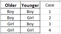
In the Jones family, all we know is that there is at least one girl. Let’s look at a diagram that shows all of the equally-likely possibilities in any family with two children:
With the Smith family, we can rule out cases 1 and 2, leaving us cases 3 and 4.
However, with the Jones family, we can only rule out case number 1. Cases 2, 3, and 4 — which are all equally likely — are all possible outcomes for the Joneses. Notice that only in case number 4 do the Jones have two daughters. So with the Joneses, the chances that there are two daughters is only 1 in 3, or 33.3%.
I had the pleasure of helping lead a field trip for 9th grade Geometry students at School Without Walls SHS that we call ‘Math on the Mall’ assisting with two colleagues from the SWW math faculty.
One of our goals is for the students to see how beautifully and geometrically this city was laid out by Pierre l’Enfant, Andrew Ellicott, and Benjamin Banneker about 230 years ago.
While there are lots of myths written and repeated about Banneker’s actual contribution, the fact is that he was the astronomer, who was responsible for determining due north, exactly, and the exact latitude and longitude of the southern tip of the original 10-mile-square piece of land. With no Internet or SatNav or even a telegraph or steam engine, but with a very nice refractor and highly accurate clock that he was entrusted with, but with no landmarks to measure from, he was able to do so, in 1790.
I was sad to see that exactly none of the students know which way was north – in a city where the numbered streets near the Mall and the rest of DC’s historic downtown were almost all laid out perfectly north-south, and the streets whose names begin with letters or words like ‘Newark’, and the streets along the Mall, are all laid out perfectly east-west. Very few of them had ever seen the Milky Way, though most had heard of Polaris or the North star.
Hopefully they will remember that in the future as they do more navigation on their own in this great city.
I challenged them to try to figure out why the angle of elevation of the North Star is the same as their latitude. Here is a diagram illustrating the problem:
The Earth, Polaris, and You.
This diagram is intended to help you understand why the North Star’s elevation above your horizon always gives you your latitude (if you live north of the Equator.
The big circle represents the Earth. The center of the earth is at E. The equator is AD.
YOU, the observer, are standing outside on a clear night. You see Polaris in the direction of ray BG. Line HCE is the Earth’s axis, and it also points at Polaris – which is so far away, and seems so tiny, but yet is also so large, that yes, parallel rays BG and CH do, for all practical purposes, point at the same point in the sky. Ray ED starts at the center of the Earth, passes through you at B, and goes on to the zenith (the part of the sky that is directly overhead). The horizon (BF) and the zenith (ray EB) are perpendicular. Also, line HCE (the earth’s axis) is perpendicular to its equator (segment AED).
Using some sort of angle measuring device, if you are out on the National Mall at night, you can very carefully measure the angle of elevation of the North Star above the local horizon, and you should ideally find that angle, FBG, is about 38.9 degrees, but we could also call it X degrees.
Prove (i.e. explain) why your latitude (which is angle AEB) measures the same as angle FBG.
Full disclosure: My daughter graduated from SWW two decades ago, and I taught there as well for a year and for 10 years at a school that is now associated with it: Francis (then JHS now a middle school).
The kids were nice back then, and they still are. I thought the teachers did a great job.
This is a DC public high school that you have to apply to.
Benjamin Banneker was an amazing person. There are a lot of myths that have been attached to his work and accomplishments, which I am guessing might be because those people didn’t actually understand the math and astronomy that he did accomplish. The best book on him is by Silvio Bedini.
‘Math on the Mall’ was originated by Florence Fasanelli, Richard Thorington, and V. Frederick Rickey around 1990. I participated as a math teacher in a couple of those tours led by FF. Later, I wanted to take my students on a similar tour that would include a trip to see a number of the works of the geometer and artist Maurice C. Escher, and couldn’t find my copy of their work, so I made up my own, and added to it using the work of FF, RT, and VFR and suggestions from teachers and students. Later on, the Mathematical Association of America made something similar, which you can find here.
My version was on the website of the Carnegie Institution for Science for a number of years. See page 56 on this link. I need to find someone to cut out some of my excess verbiage and then trot it out to a publisher.