
I’ve captured some variable stars, both with somebody figuratively holding my hand at almost every step of the way, 22 years ago, at a 2-week summer session at Mount Wilson that I highly recommend, and also with a Seestar S50, after failing a few times.
I was hoping to be able to finally capture an exoplanet transit. I tried in a couple of different ways on the night of January 18-19, but failed. Even so, I count the night as a major success.
It turned out that there were four (yes, 4!) different exoplanets that were supposed to have transits quite visible, during the same night, from my location (Hopewell Observatory in northern Virginia), and I was going to be staying up there all night anyway, with some others.
I used the Plan mode of my Seestar to take 30-second exposures of the star that looked like it would be the easiest to capture, namely HAT-P-32, which is in Andromeda at Right Ascension 02h 04m 10.00s and Declination +46° 41` 16.00″, It was supposed to have a depth of transit (or coverage of the star by the planet) of 22.2 parts per thousand, or 2.22%, which I thought sounded like quite a bit.
Unfortunately, it’s not very much at all, at least in terms of star magnitudes!
Perhaps you knew (I had forgotten it) the formula for turning brightness changes into magnitude changes.
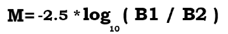
(M is the magnitude change, B1 is the actual measured flux of photons at time 1 or from star 1, and B2 is the same flux, measured the same way, at time 2 or from star 2.)
You don’t even need to remember what a logarithm is to punch this into your calculator. I found that if you make it so that the ratio of B1 to B2 is one-half, you get a result of 0.75257… and if you try it the other way around, you get the exact same result, with a negative sign in front.
Let’s see: a drop in brightness of 22.2 parts per thousand leaves 977.8 parts per thousand still reaching my telescope. So my B1 needs to be 977.8 and B2 needs to be 1000. Or I could just type -2.5*log(0.9778) and when I do that, I get a drop in magnitude of 0.023, which is not very much at all!
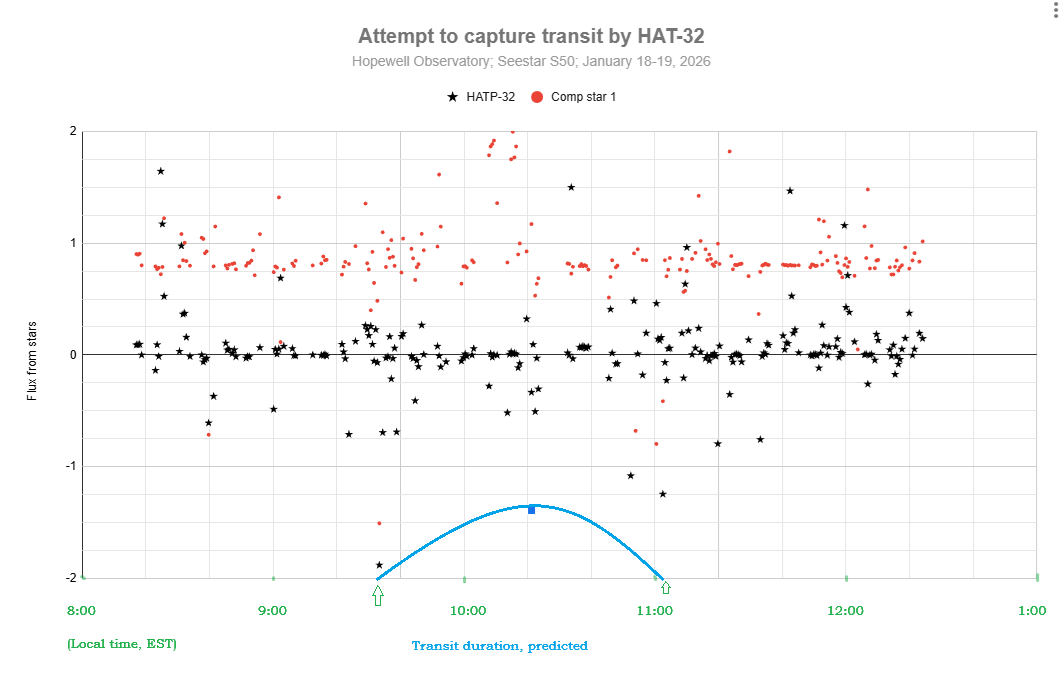
Well, here is my attempt at detecting a transit for HAT-P-32b. I don’t see any sign of a transit. Do you? Part of the problem may have been that my target star was in the trees for part of the time…
It appears that others have succeeded at this:
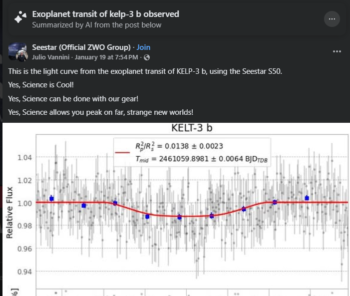
I will hope for better weather, better preparation of every step, and fewer tree branches next time!
By the way, here is my workflow. Steps 0 – 2 should be done at home, inside, in comfort, well before leaving for your observing site.
0. You must have both SeeStar and plate solving software (and its databases) operational on your computer. Download and install you have SeeStar, AstroImageJ, Astronometry.net and all of the databases for these accessible on your computer. You can also use ASTAP if you prefer for plate-solving, but AIJ uses Astronometry.net.
- Look up which exoplanets are supposed to be visible in your area on the Swarthmore database, for how long, and in what part of the sky. Pick the best ones, with the greatest change in brightness. Print out the data.
2. Connect your Seestar to your tablet or smartphone and create a Plan to image that star for the entire time, with 30 second exposures, no filters, saving every frame. Double-check all your settings! You can do one target after the other, sequentially, but with the current SeeStar software, it doesn’t appear that you can ask it to rotate among several targets for a period of time. If you want to study variable stars, you might find that the Seestar’s pixel wells will get saturated with too many photons, which renders all your time and data is useless. To stop the saturation, set the exposures to as short as possible (10 second exposures), and set the light-pollution filter. If it’s still saturated, you might even need a sub -aperture mask to cut the signal further. You may or may not find that you have to manually change settings at various times during the night; if so, set an alarm for yourself.
3. Later, at the observing site, after sundown: Level your tripod, attach Seestar, turn it on, arrange for a power supply for it, use Bluetooth connect the same tablet or smartphone that you used to make the plan, and tell Seestar to start implementing your Plan. Check the clock and the smart device to make sure Seestar has actually started carrying out the plan. Periodically, re-check to make sure the images look decent. (I have found that Seestar is actually very good at centering your target precisely where you asked it to go to!
4. Let the Seestar do its thing. Check the image that shows up in ‘Star Gazing’ every so often. That window shows you the latest version of the stacked and calibrated image – which you won’t need for attempting to catch an exoplanet transit — not the current sub-exposure.
5. The next morning, in comfort, use a USB-C cable to connect your Seestar to a computer. Use a finder to locate the My Works folder on the Seestar, and find the folder that has all of your subs (frames). They should be in ASIF format. If you like, you can upload them to your computer, or else you can leave them on the Seestar. Take your pick.
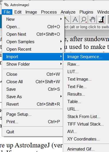
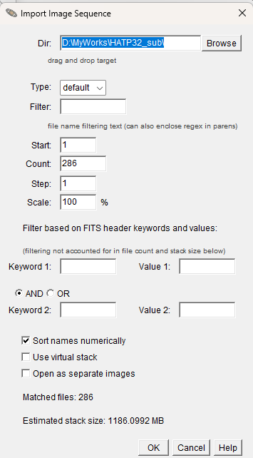
6. Fire up AstroImageJ (version 6) on your computer. Use File/Import Sequence to load that same sequence of subs that you just found. Keep in mind that some parts of the process (especially plate solving) might tie up your computer for a long time, perhaps hours. I would suggest only importing every 10th sub, to begin with, to find out if the whole stack of images is garbage or useful. If desired, you can always import the entire stack later. If I change the Step to 10, it will instead load image #1, then #11, then #21, and so on…
6. Inspect the images, and make a note of the ones you think are garbage. Get rid of those subs.
7. Then have AIJ do a plate-solve by chosing WCS (World Coordinate System) then Plate Solve with Astronometry.net (With Options). One of those options should be the coordinates of your star, which you should type in manually. You will need an Astronometry.net user key. You may use mine if you want: tyqwnsiwmabnvdlt. Make sure that Autosave and Skip Images With WCS are Enabled. When you have all that done, click on ‘Start’.
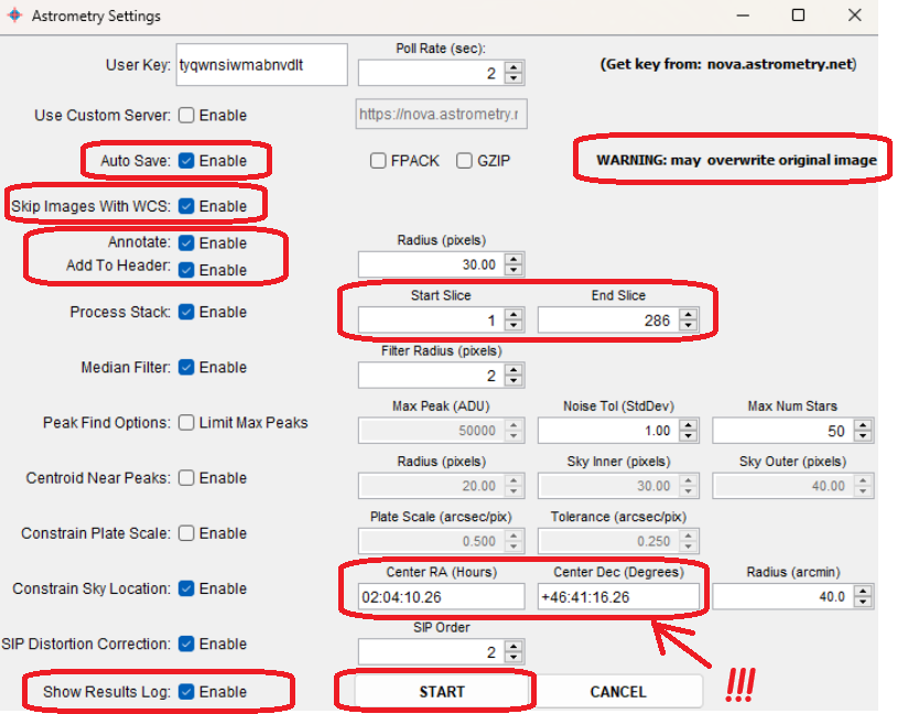
AIJ and Astrometry will then do their best to figure out exactly where the image was in the sky, and will record the RA and Dec of every single object in it and add that to the FITS header. AIJ&A will also indicate which are the cardinal directions. Hopefully, they will be able to solve every image. If Astrometry.net fails, you can try doing the same thing with ASTAP instead, which is insanely fast.
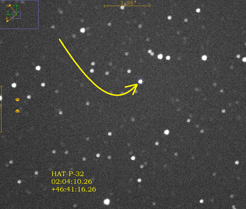
8. Once all of your images have been plate solved, then enlarge one of the images and find your star by checking the coordinates very carefully by moving your mouse around on the image. Since your image has been plate-solved, AIJ now knows exactly how to match the pixels on your screen to the coordinates in the sky, which is extremely impressive! (Try doing that yourself, by eye!) Pay attention to the ‘North” and “East” arrows. North is in the positive declination direction (degrees), and east is the positive right ascension direction (hours). Zoom in to your star, and then do a screen-snip and save it to some other app, and draw arrows showing exactly which star is the one you want, like I did here for my star, HAT-P-32. I also typed in its coordinates. This is for your own reference.
9. The next step is to have the computer compare the brightness of your selected star with a dozen or so comparison stars, and to do so in every frame (or ‘slice’ or ‘sub’), and show you the results in table (spreadsheet) form, and as a graph (chart) of the brightnesses over time of as many of the stars as you like. AIJ does this incredibly well, and incredibly quickly1 You don’t have to go frame by frame, measuring the brightness by eye of each and every single selected star, and noting any changes in brightness, by hand, as was done a century ago or so, in the days of photographic emulsions on thin glass plates. Here is a method for doing it in AIJ:
10. So what on earth is it doing, and how does it measure comparative brightness? My understanding is that it draws a three circles of increasing radii around each star, as I show here:
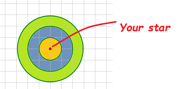
Basically, the software counts all the photons that it captures inside the first ring, which I labeled in yellow. It produces a number: the full width half max. Then it does the same thing for the photons in the outer ring, which it then assumes is the background brightness. I shaded this ring as olive green. It subtracts the FWHM for the yellow ring minus the FWHM of the green ring. It also compares those numbers for all of the comparison stars, and displays all the data in a variety of ways, including a spreadsheet and a graph.
11. Unfortunately, I found that I was unable to get AIJ to make very useful graphs, so I exported the entire spreadsheet into Excel and Google Sheets and made my graphs there.
Here is a link to a much better article on doing much the same thing:
