I’d like to share these spectacular images of our Sun, taken by Prasad Agrahar with his home-made spectroheliograph.
His first image is at H-alpha (656 nm), second is at H-beta (486 nm), and the third is at Helium D3 (585 nm).
With this device, IIUC, he can make an image at just about any wavelength that makes it through the front lens of the optics. He posted this to the NCA email list.
DIY!!
Guy Brandenburg
Prasad wrote:
Here are three images of our Sun, taken on Thursday morning with my DIY spectroheliograph. The weather was quite windy, and the seeing was poor.
The above is H-alpha with [sunspot groups] AR 4294 and 4296 dazzling.
This is H-beta
And finally,
The above image is (…) Helium-D3, the emission line at 5875A.
Most (but not all) of the variable stars I tried over the past month or so were simply too bright for this sensor. The target stars were saturated (ie some of the pixels’ electron wells simply overflowed) despite using the shortest available exposure, adding the light pollution filter and refocusing. Seestar won’t let your change the ISO nor open the shutter for less than 10 seconds.
I did get some believable light curves on BE Lyncis (aka HD67390)and U Cephii (aka HD 5679). I attack some graphs I made.
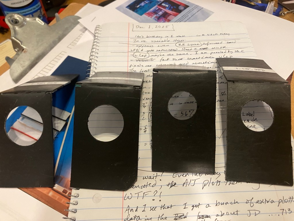
I used some black plastic I had,and my set of Forster bits, to make holes of sizes 1”, 1-1/8”, 1-1/4”, and 1-1/2”, in case I want to try brighter variable stars again like RR Lyrae.
I very impressed that Seestar absolutely nails the locations of every single one of these targets! I’m also pleased that AstroImageJ allows quick and easy plate-solving!
I went up to Hopewell on Wednesday night, and practiced once again taking images of RRLyrae with my Seestar S50, but this time with the built-in light-pollution rejection filter in place. I figured that would reduce the number of photons by a lot, and maybe by enough to stop overwhelming the pixels.
Unfortunately, it was not sufficient, so, since I cannot reduce the number of seconds of exposure for each sub-image (or ‘slice’ as AstroImageJ calls them) below 10, and I cannot change the ISO or gain for the chip, the only choices left are, in order of ease of implementation:
De-focus the images to spread the photons into a wider range of pixels, hopefully not causing any of them to become saturated, but not so much as to confuse the plate-solving app;
Make a black, circular mask smaller than 50 mm in diameter and put it in front of the lens, reducing the total number of photons;
Persuade the engineers and programmers at ZWO to change the software to allow users to reduce the length of exposures, and to allow time lapse photography with what they call Star-Gazing but everybody else calls deep-space observing.
Number 1 I will do next time.
By the way, the exact mechanism by which this variable star dims and brightens is still not fully understood, though its timing cycle is extremely regular and quite well known.
No Auroras for me:
It was very cold and windy so I couldn’t stand being outside up on the Bull Run Mountain ridge for very long at a time. The sky was almost perfectly clear the entire night, and the beautiful winter constellations were extremely bright, and it was fun watching them make that apparent great pivot around us.
I saw no auroras; since I was was groggy (from forgetting my meds) and quite cold, so I spent most of the night inside napping and trying to get warm, but went out from time to time to look around and to check on the progress of my little Seestar. So when the peak happened I was probably dozing. Not too many other folks saw it, apparently, and the images I’ve seen were not nearly as impressive as for other aurorae on other dates. Oh, well.
As described in my last post, I got a light curve for a known variable star in my little Seestar S50 a few weeks ago that showed absolutely no variability whatsoever over a roughly 4 hour period. Since this star’s variation occurs extremely regularly, there is a known formula that will give you the precise location in its cycle if you feed in the Julian day (JD). I plugged the start and end times for my run, and got the following:
And was confused
So RRLyrae should have dropped from something near 7.3 magnitude to around 7.6 magnitude, which is a LOT for this sort of thing. But my graph of brightness of RRLyae, compared to a nearby star of roughly the same magnitude, looks like this:
Which is barely any change at all. The few pairs of dots below the blue blob line are glitchy data that should be ignored; notice that it happens for both stars. In fact, I see more variability in the pink comparison star’s brightness than I do with RRRLyrae.
Was the scope indeed pointed at the correct star? Well, I had plate solving on each and every frame, and they all agreed, so, yes.
I did notice a problem with saturation, but didn’t know exactly by how much. Nikolaos Bafitis suggested that I use my mouse to look more closely at the centers of the star images themselves in AstroImageJ. I did so, and at last noticed that one of the boxes held the number of pixel counts right under my mouse pointer. Duh! Sure enough, my target star, RR Lyrae, had a count of 65,533, which is 2^16, and (I looked it up) that is precisely the maximum for these pixels on these CMOS cameras. So that’s why RR Lyrae’s brightness was so steady: it was always OVERFLOWING.
So I have to figure out a way to gather fewer photons per pixel around the target and comparison stars. There are several possible ways of doing so without changing the electronics or trying to mess with the operating system or user interface.
Reduce the ISO setting from the current default value.
Shorten the exposure time.
Change the focal ratio by placing a circular mask over the lens aperture.
De-focus the images so that the light is spread out over a larger area.
Add some sort of filter.
Unfortunately right now, the Seestar doesn’t allow you to do either number 1 or number 2. It would be nice if ZWO engineers would add those capabilities in the ‘advanced’ menu,
Number 3 is quite doable. I happen to have on hand a large roll of black Kydex plastic and a set of Forstner bits to make nice holes with. But it this would require a fair amount of time and effort. It would also reduce the resolution of an already rather small 50mm lens.
Number 4 is more easily doable: turn off the autofocus feature and do some experimentation to find a good fixed de-focus point. However, if the stars are too fuzzy, then plate-solving becomes much harder and slower.
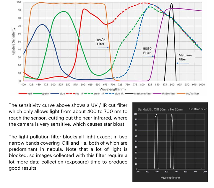
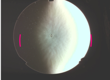
Number 5 can be done by using the built-in light pollution filter, whose transmission bandwidth is very small. It’s the bottom graphic below.
The graphics above come from an excellent Unofficial Seestar handbook written by Tom Harnish. He has a number of suggestions that I hope the engineers at ZWO pay attention to and follow.
The option that seems easiest is number 5, using the light pollution filter. If I couple that with the built-in time-lapse feature, I won’t fill the Seestar’s entire memory with a zillion FITS images.
I hope to try this tonight up at Hopewell Observatory, where I can set this up, have it run all night connected to mains power, and I can sleep in a nice warm cabin.
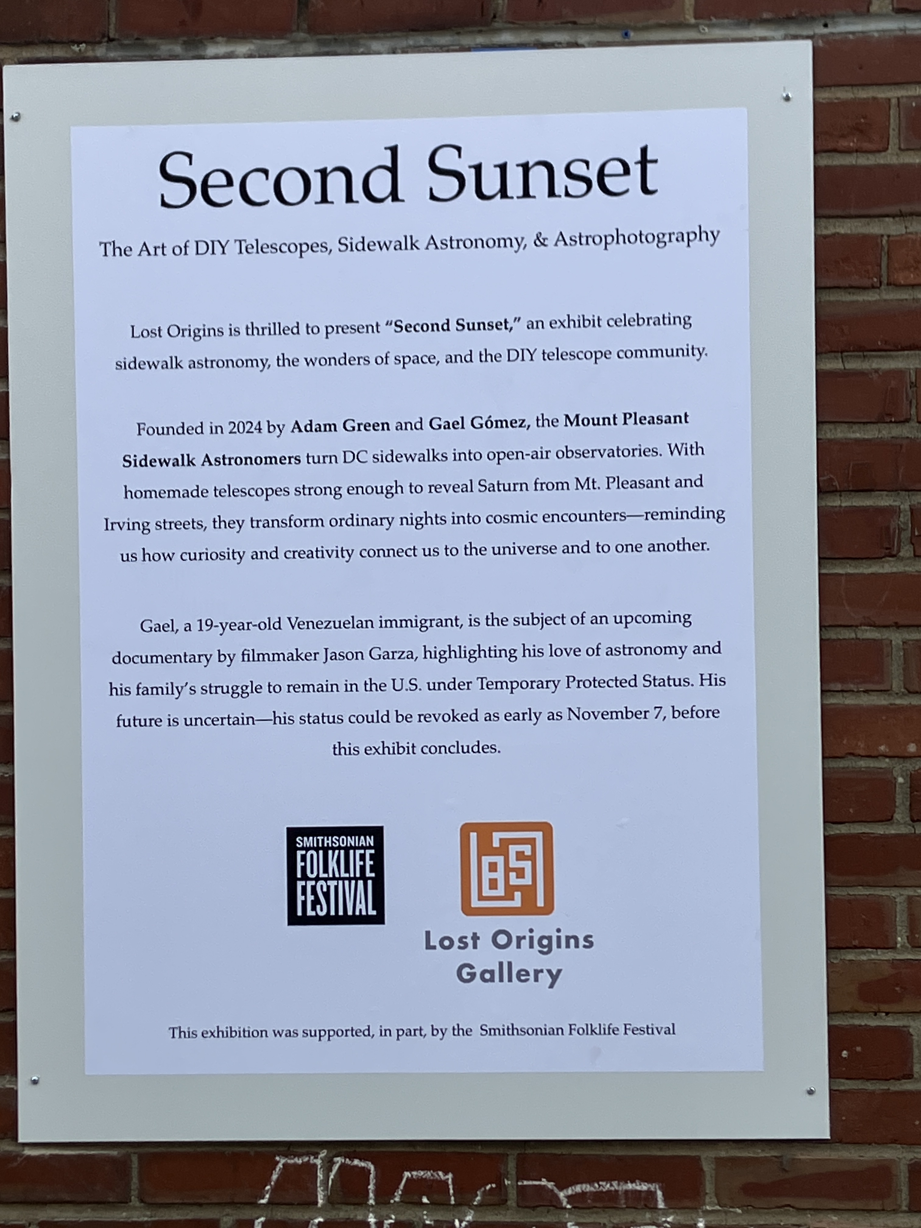
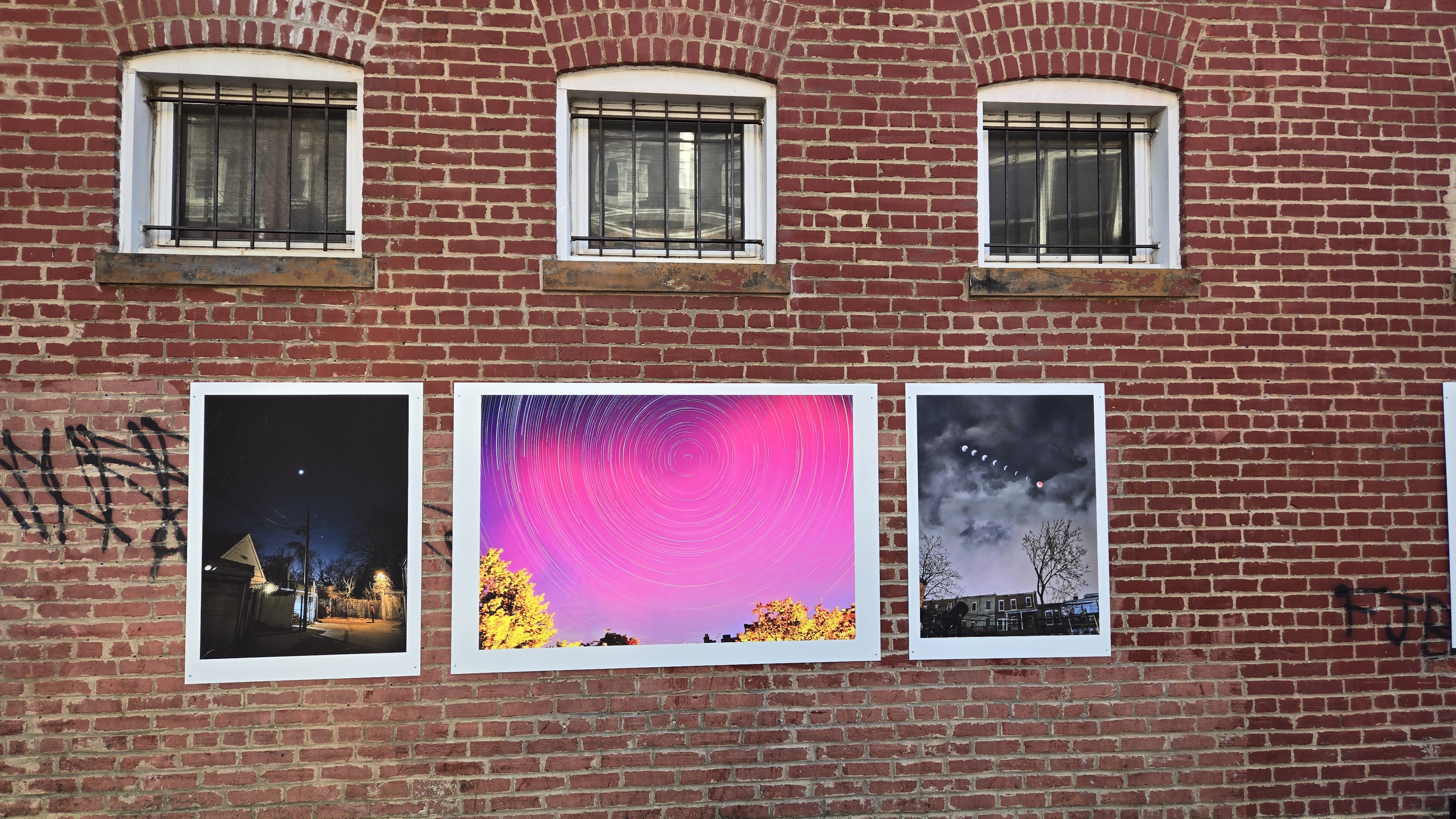
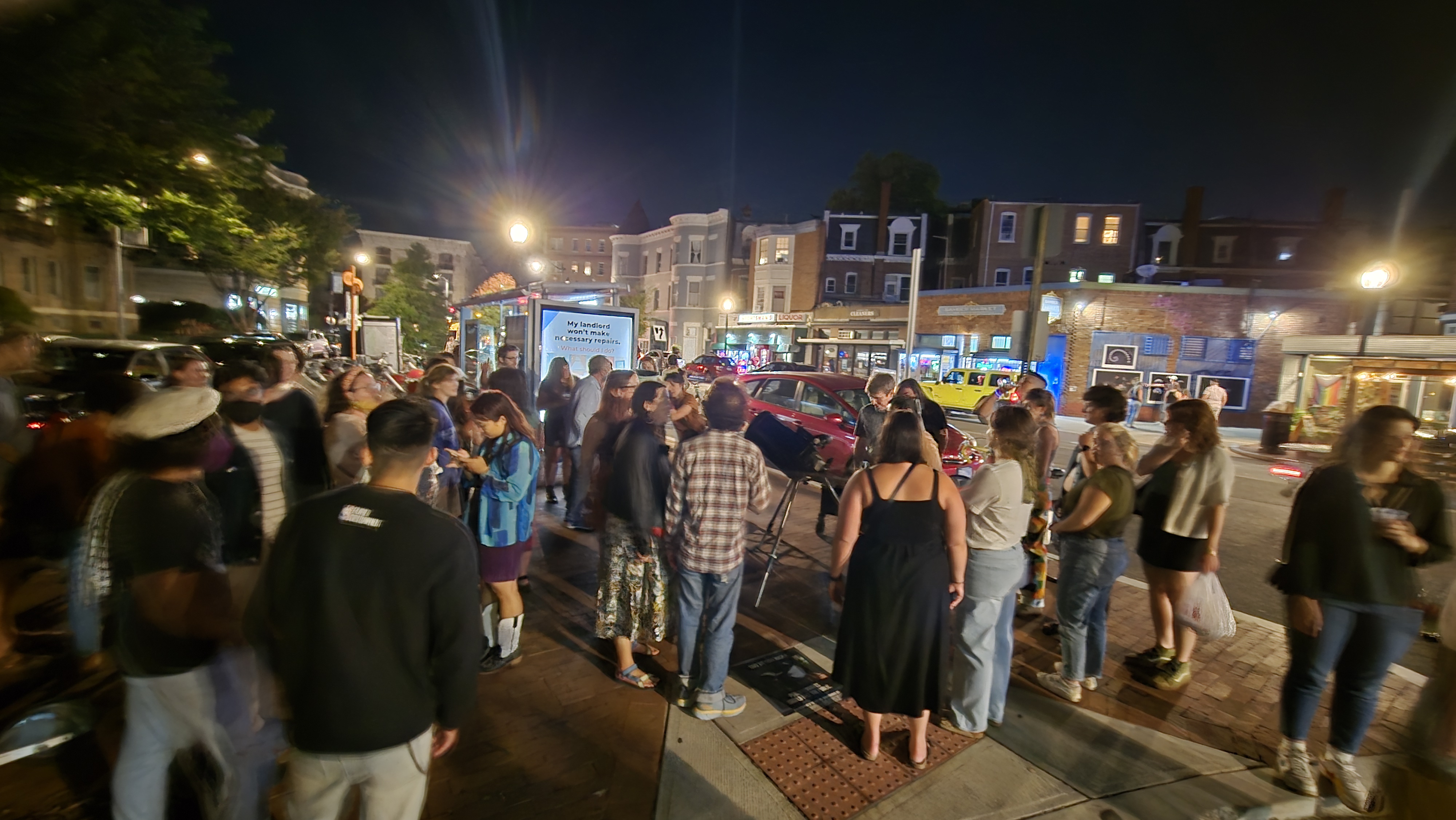
Last night was the opening of an exhibit called Second Sunset in an alley off Mt Pleasant Triangle in NW DC. Great astrophotos by 19-year old Gael Gomez, his neighbor Adam Green, and NCA VP Bryan Vandrovec! The images are huge – four to six feet across, and printed on durable sandwiches of aluminum and plastic, so they will survive outside for months. They were printed by Jason Hamacher of Lost Origins Gallery, located about a block away, aided in part by the Smithsonian’s Folk Life Festival.
It coincided with the 3rd annual Art All Night – Mount Pleasant, so a LOT of people were out having a good time, listening to a live Colombian band and visiting dozens of vendors and exhibits under tent covers on the Triangle.
So when Gael and Guy Brandenburg (NCA president) brought out their telescopes on the other side of Mt Pleasant Street, once we could actually see a few stars, we had long lines of people waiting patiently to look at double stars, Saturn, the ISS, and the Moon, and then discussing what they had seen, right up until 11:30 PM. We all had a blast!
If you can’t read the text, it says, “The Art of DIY Telescopes, Sidewalk Astronomy, and Astrophotography: The Debut Exhibit of the Mt Pleasant Sidewalk Astronomers”. As well as “Lost Origins Outside” and “November 12 to November 9, 2025.”
Captions are coming for all of the photos, explaining how they were made and what they depict, as well as a sign explaining the National Capital Astronomers which has been running the DC DIY telescope workshop since World War 2, in which both Guy and Gael made their first telescopes.
We only truly discovered the nature of galaxies, of nuclear fusion, and of the scale of the universe a mere century ago.
Dark matter was discovered by Vera Rubin just over 40 years ago and dark energy a few years later, just before the time that both professional and amateur astronomers began switching over to CCD and later CMOS sensors instead of film
The first exoplanet was discovered only 30 years ago, and the count is now up to almost six thousand of them (as of 1/21/2024).
While multi-billion dollar space telescopes and giant observatories at places like Mauna Kea and the Atacama produce the big discoveries, amateur astronomers with a not-outrageous budget can now afford to purchase relatively small rigs armed with excellent optics and complete computer control, and lots of patience and hard work, can and so produce amazing images like the ones here https://www.novac.com/wp/observing/member-images/ or this one https://www.instagram.com/gaelsastroportrait?igsh=cjMzYWlqYjNzaDlw, by one of the interns on this project. Gael’s patience, cleverness, dedication and follow-through are all praiseworthy.
However, it is getting harder and harder every year for people to see anything other than the brightest planets, because of ever-increasing light pollution; the vast majority of the people in any of the major population centers on any continent have no hope of seeing the Milky Way from their homes unless there is a wide-spread power outage. Here in the US, such power outages are rare, which means that if you want to go out and find a Messier object, you pretty much cannot star-hop, because you can only see four to ten stars in the entire sky!
One choice is to buy a completely computer-controlled SCT like the ones sold by Celestron. They aren’t cheap, but they will find objects for you.
But what if you don’t want another telescope, but instead want to give nice big Dobsonian telescope the ability to find things easily, using the capabilities inside one’s cell phone?
Some very smart folks have been working on this, and have come up with some interesting solutions. When they work, they are wonderful, but they sometimes fail for reasons not fully understood. I guess it has something to do with the settings in the cell phone being used.
The rest of this will be on one such solution, a commercial one called StarSense from Celestron that holds your phone in a fixed position above a little mirror, and you aim the telescope and your cell phone’s camera at something like the top of a tower far away. Then it uses both the interior sensors on your cell phone and images of the sky to figure out where in the sky your scope is pointing, and tells you which way to push it to get to your desired target.
When it works, it’s great. But it sometimes fails.
You have to buy an entire set from Celestron – one of their telescopes (which has the gizmo built in) along with the license code to unlock the software.
You supply the cell phone.
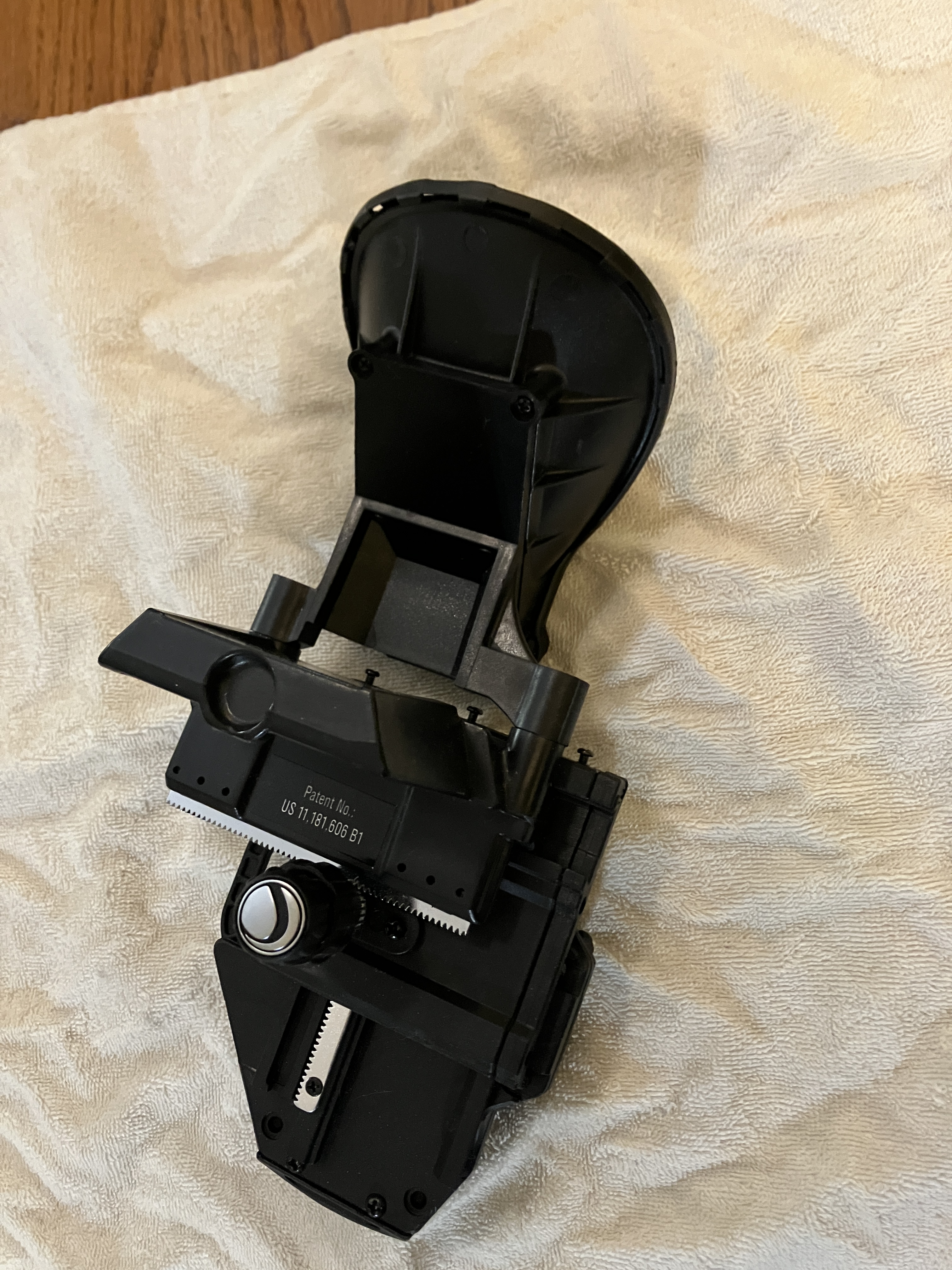
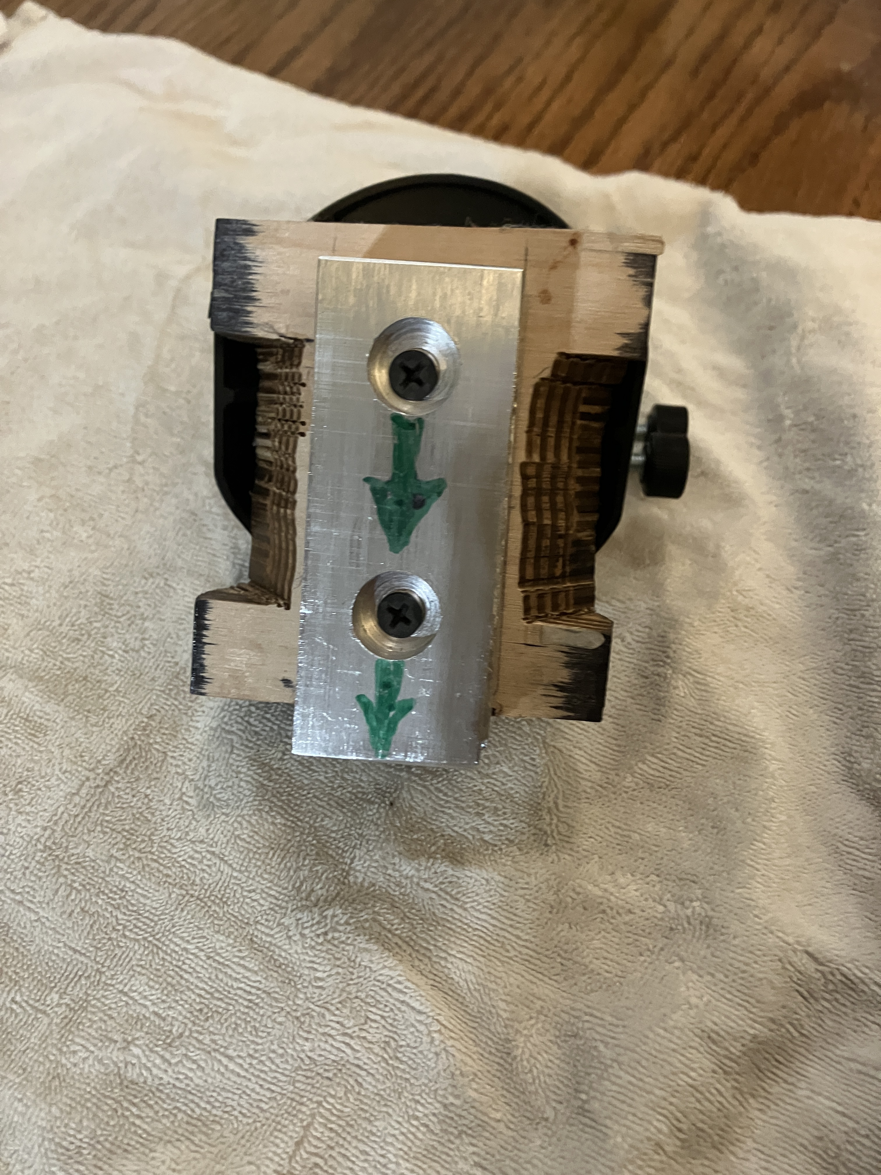
The entire setup ranges in price from about $200 to about $2,000. You cannot just buy the holder and the code from them; you must buy a telescope too. I already had decent telescopes, which I had made, so I bought the lowest-priced one. I then unscrewed the plastic gizmo, and carved and machined connection to a male dovetail slide for it. I also fastened a corresponding female dovetail to each of my scopes. The idea was to then slip this device off or onto whichever one of my telescopes is going to get used that night, as long as I that has a vixen dovetail saddle, and put inexpensive saddles on several scopes I have access to.
Here are some photos of the gizmo:
NCA’s current interns (Nabek Ababiya and Gael Gomez) and I were wondering about the geometry of the angles at which StarSense would aim at the sky in front of the scope. My guess had been that Celestron’s engineers would make the angles of their device so that the center of the optical pencil hitting the lens dead-on at 90 degrees, and hence coning to a focus at the central pixel of the CMOS sensor, would be parallel to the axis of the telescope tube.
We didn’t want to touch the mirror, because it’s quite delicate. But as a former geometry teacher, I couldn’t leave this one alone, so along with Gael and Nabek I made some diagrams and figured out what the angles had to be if the axis of the StarSense app’s image were designed to be precisely parallel to the axis of the telescope.
In my diagram below, L is the location of the Lens, and IJCK is the cell phone lying snug in its holder. The user can slide the cell phone left and right along that line JD as we see it here, or into out of the plane of the page, but it is not possible to change angle D aka <CDE – it’s fixed by the factory molds to be some fixed angle that we measured with various devices to be 19.0 degrees.
Here is a version of the diagrams we made that showed what we predicted all the angles would be so that optical axis OH will be parallel to the tube axis EBD, and that lens angle ILH is a right angle. We predicted that the mirror’s axis would need to be tilted upwards by an angle of 35.5 degrees (anle HBD).
To our surprise, our guesses and calculations were all wrong!
After careful measurements we found that Celestron’s engineers apparently decided that the optical axis of the SS gizmo should instead aim the cell phone’s camera up by 15.0 degrees (angle BGH below). The only parallel lines are the sides of the telescope tube!
We used a variety of devices to measure angle FBD and MNC to an accuracy of about half a degree; all angles turned out to be whole numbers.
Be that as it may, sometimes it works well and sometimes it does not.
Zach Gleiberman and I tested it on an open field in Rock Creek Park here in DC back in the fall of 2024, using the Hechinger-blue 8 inch dob I made 30 years ago and still use. We found that SS worked quite well, pointing us quite accurately to all sorts of targets using my iPhone SE. The sky was about as good as it gets inside the Beltway, and the device worked flawlessly.
Not too long afterwards, I decided to try out an Android-style phone (a REVVL 6 Pro) so that I wouldn’t have to give up my cell phone for the entire evening at Hopewell Observatory. I was unpleasantly surprised to find that it didn’t work well at all: the directions were very far off. I thought it might be because the scope in question had a rather wide plywood ring around the front of its very long tube, and that perhaps too much of the field of view was being cut off?
Why it fails was not originally clear. I thought nearly every modern phone would work, since for Androids, it just needs to be later than 2016 and have a camera, an accelerometer, and gyros, which is a pretty low bar these days. However, my REVVL 6 Pro from T-Mobile is not on the list of phones that have been tested to work!
Part of my assumption that the axis of the SS gizmo would be parallel to the axis of the scope was an explanation that StarSense on had such a large obstruction in front of the SS holder, in the form of a wide wooden disk reinforcing the front of a 10″ f/9 Newtonian, that the SS was missing part of the sky. We now know that’s not correct. It’s an interface problem (ie software) problem.
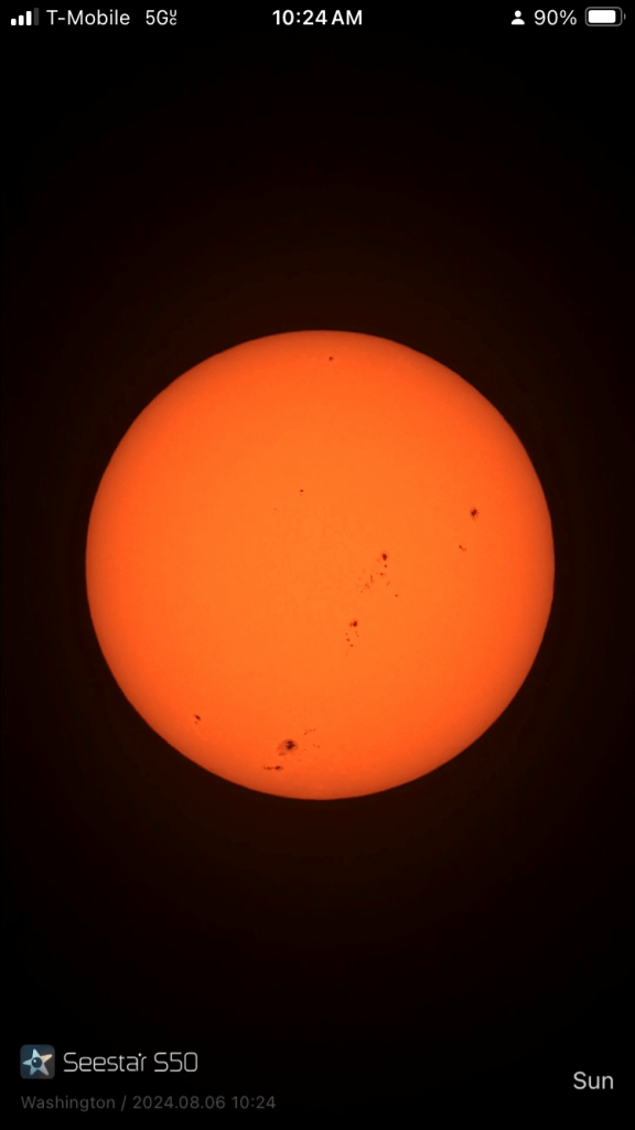
Look what this little thing can do that I’ve always failed at myself, even with an entire observatory at my disposal: take decent astrophotos.
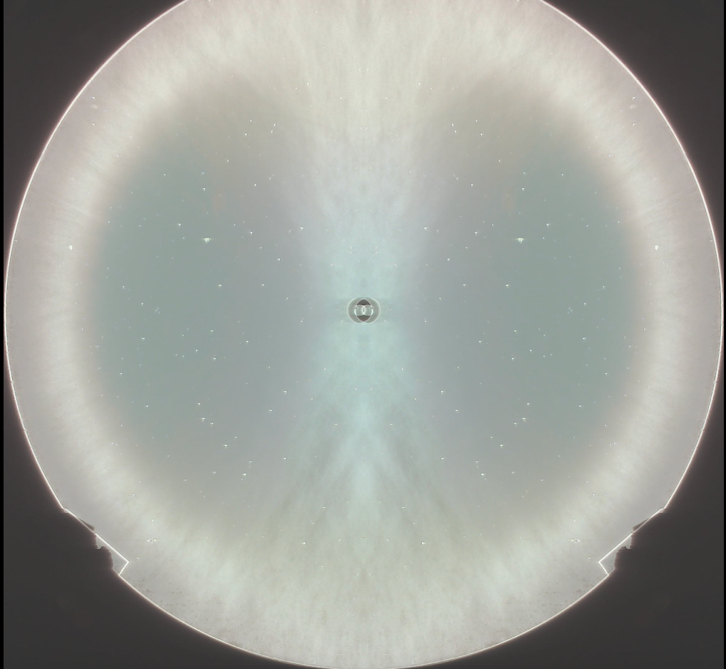
Here it is on a home made tripod, taking photos of the sun. Notice the reflective solar filter. Here are two images:
The device woke up, and after less than a minute of self’s-calibration, it pointed very accurately at the sun and focused itself perfectly. It produces a continuous feed; I even did 100 frames of a time-lapse. It’s all stored on my cell phone but I can share the photos or even live views with folks nearby.
And from night time spots here in DC and NOVA:
This can take tolerable astrophotos even when surrounded by streetlights!
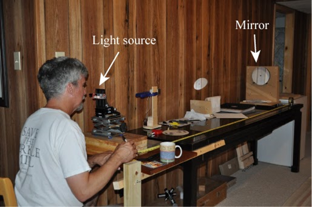
For many years now, I have been trying and (mostly) failing at using some sort of digital camera when testing the optics of the mirrors we fabricate and evaluate at the ATM workshop at the Chevy Chase Community Center here in DC.
I can now report that there finally is some useful and non-vignetted light at the end of the testing tunnel!
Foucault, knife-edge image, raw
Same mirror, at a different longitudinal location, image flipped right to left (ie across the y-axis), and then pasted onto the original image
Same mirror, same location as the image directly above, with circles and measurements added in Geometer’s Sketchpad
I used an old Canon FD film camera lens (FL=28 mm) that I got about 40 years ago and haven’t used in several decades to get a bunch of really nice knife-edge images of a 16″ Meade mirror, located on a stage that can be moved forward and back in whatever steps I like by a smartphone app and a stepper motor setup that Alan Tarica and Pratik Tambe designed and put together.
Just now, I finally figured out how to use IrfanView to take one of the images, flip it left-to-right (that is, across the y-axis) and superimpose one onto the other with 50% transparency. A bright ring appeared, which shows the circular ring or zone where the light from our LED, located just under the camera lens, goes out to the mirror and bounces directly back to the lens and is captured by the sensor as a bright ring.
I then captured and pasted that image into Geometer’s Sketchpad, which I used to draw and measure the radii of two circles, centered at the doughnut marking the center of the mirror. This is a somewhat crude measurement of the radii, but it appears that this zone is is at 83% of the diameter (or radius) of the original disk, which is 16 inches across.
Now I just need to do the same thing for all of the other images, and then correlate the radii of the bright zones with the longitudinal (z-axis) motion of the camera and stand, and I will know how close this mirror is to a perfect paraboloid.
There is an app that supposedly does this for you, called Foucault Unmasked, but it doesn’t seem to work well at all. As you can see from these images, FU is unable to find zones that are symmetrically placed on either side of the center of the mirror. I don’t know what algorithm FU uses, but it sure is f***ed up.
Foucault Unmasked thinks that those two red marks are the zone being measured here. It’s pretty hard to be more wrong than that.
Again, FU at work, badly. Not quite as awful as the previous one, but still quite useless!
Thanks a lot to Tom Crone, Gert Gottschalk, Pratik Tambe, Alan Tarica, and Alin Tolea for their help and suggestions!
Several people have helped me with this applied geometry problem, but the person who actually took the time to check my steps and point out my error was an amazing 7th grade math student I know.
It involves optical testing for the making of telescope mirrors, which is something I find fascinating, as you may have guessed. Towards the end of this very long post, you can see the corrections, if you like.
Optics themselves are amazingly mysterious. Is light a wave, or a particle, or both? Why can nothing go faster than light? We forget that humans have only very recently discovered and made use of the vast majority of the electromagnetic spectrum that is invisible to our eyes.
But enough on that. At the telescope-making workshop here in DC, I want folks to be able to make the best ordinary, parabolized, and coated mirrors possible with the least amount of hassle possible and at the lowest possible cost. Purchasing high-precision, very expensive commercial interferometers to measure the surface of the mirror is out of the question, but it turns out that very inexpensive methods have been developed for doing that – at least on Newtonian telescopes.
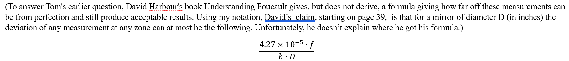
Tom Crone, a friend of mine who is also a fellow amateur astronomer and telescope maker, wondered how on earth we can report mirror profiles as being within a few tens of nanometers of a perfect paraboloid with such simple devices as a classic Foucault knife-edge test.
He told me his computations suggested to him that the best we could do is get it to within a few tenths of a millimeter at best, which is four orders of magnitude less precise!
I assured him that there was something in the Foucault test which produced this ten-thousand-fold increase in accuracy, but allowed that I had never tried to do the complete calculation myself. I do not recall the exact words of our several short conversations on this, but I felt that I needed to accept this as a challenge.
When I did the calculations which follow, I found, to my surprise, that one of the formulas I had been taught and had read about in many telescope-making manuals, was actually not exact, and that the one I had been told was inherently less accurate, was, in fact, perfectly correct! Alan Tarica sent me an article from 1902supposedly explaining the derivation of a nice Foucault formula, but the author skipped a few bunch of important steps, and I don’t get anything like his results. it took me a lot of work, and help from this rising 8th grader, to find and fix my algebra errors. I now agree with the results of the author , T.H.Hussey.
I am embarrassed glad to say that even after several weeks of pretty hard work, an exact, correct formula for one of the commonly used methods for measuring ‘longitudinal aberration’ still eludes me. was pointed out to me by a student who took the time to Let’s see if anybody can follow my work and helped me out on the second method.
But first, a little background information.
Isaac Newton and Leon Foucault were right: a parabolic mirror is the easiest and cheapest way to make a high-quality telescope.
If you build or buy a Newtonian scope, especially on an easy-to-build Dobsonian mount, you will get the most high-quality photons for the money and effort spent, if you compare this type with any other type of optics at the same diameter. (Optical designs like 8-inch triplet apochromats or Ritchey-Chrétiens, or Maksutovs, or modern Schmidt-Cassegrains can cost many thousands of dollars, versus a few hundred at most for a decent 8″ diameter Newtonian).
With a Newtonian, you don’t need special types of optical glass whose indices of refraction and dispersion, and even chemical composition, must be known to many decimal places. The glass can even have bubbles and striations, or not even be transparent at all! Any telescope that only has mirrors, like a Newtonian, will have no chromatic aberration (ie, you don’t see rainbows around bright stars) because there is no refraction – except for inside your eyepieces and in your eyeball. All wavelengths of light reflect exactly the same –but they bend (refract) through glass or other materials at different angles depending on the wavelength.
Another advantage for Newtonians: you don’t need to grind and polish the radii of curvature of your two or three pieces of exotic glass to exceedingly strict tolerances. As long as you end up with a nice parabolic figure, it really doesn’t matter if your focal length ends up being a few centimeters or inches longer or shorter than you had originally planned. Also: there is only one curved mirror surface and one flat one, so you don’t need to make certain that the four or more optical axes of your mirrors and/or lenses are all perfectly parallel and perfectly concentric. Good collimation of the primary and secondary mirrors to the eyepiece helps with any scope, but it’s not nearly as critical in a Newtonian, and getting them to line up if they get knocked out of whack is also much easier to perform.
With a Newtonian, you only need to get one surface correct. That surface needs to be a paraboloid, not a section of a sphere. (Some telescopes require elliptical surfaces, or hyperbolic or spherical ones, or even more exotic geometries. A perfect sphere is the easiest surface to make, by the way.)
In the 1850’s, Leon Foucault showed how to ‘figure’ a curved piece of glass into a sufficiently perfect paraboloid and then to cover it with a thin, removable layer of extremely reflective silver. The methods that telescope makers use today to make sure that the surface is indeed a paraboloid are variations and improvements on Foucault’s methods, which you can read for yourself in my translation.
Jim Crowley performing a Foucault test
It turns out that the parabolic shape does need to be very, very accurate. In fact, over the entire surface of the mirror, other than scratches and particles of dust, there should be no areas that differ from each other and from the prescribed geometric shape by more than about one-tenth of a wavelength of green light (which I will call lambda for short), because otherwise, instead of a sharp image, you just receive a blur, because the high points on the sine waves of the light coming to you would tend to get canceled out by the low points.
Huh?
Let me try to explain. In my illustrations below, I draw two sine waves (one red, one green) that have the same exact frequency and wavelength (namely, two times pi) and the same amplitude, namely 3. They are almost perfectly in phase. Their sum is the dark blue wave. In diagram A, notice that the dark blue wave has an amplitude of six – twice as much as either the red or green sine wave. This means the blue and green waves added constructively.
Next, in diagram B, I draw the red and green waves being out of phase by one-tenth of a wave (0.10 lambda) , and then in diagram C they are ‘off’ by ¼ of a wave (0.25 lambda). You will notice that in the diagrams B and C, the dark blue wave (the sum of the other two) isn’t as tall as it was in diagram A, but it’s still taller than either the red or green one.
One-quarter wave ‘off’ is considered the maximum amount of offset allowed. Here is what happens if the amount of offset gets larger than 1/4:
In diagram D, the red and green curves differ by 1/3 of a wave (~0.33 lambda), and you notice that the blue wave (which is the sum of the other two) is exactly as tall as the red and green waves, which is not good.
Diagram E shows what happens is what happens when the waves are 2/5 (0.40 lambda) out of phase – the blue curve, the sum of the other two, now has a smaller amplitude than its components!
And finally, if the two curves differ by ½ of a wave (0.5 lambda) as in diagram F, then the green and red sine curves cancel out completely – the dark blue curve has become the x-axis, which means that you would only see a blur instead of a star or a planet. This is known as destructive interference, and it’s not what you want in your telescope!
But how on earth do we achieve such accuracy — one-tenth of the wavelength of visible light (λ/10) over an entire surface? And if we do, what does it mean, physically? And why one-tenth λ on the surface of the mirror, when ¼ λ looked pretty decent? For that last question, the reason is that when light bounces off a mirror, any deviations are multiplied by 2. So lambda – about 55 nanometers or 5.5×10^(-8) m- is the maximum allowable depth or height of a bump or a hollow across the entire width of the mirror. That’s really small! How small? Really insanely small.
Let’s try to visualize this by enlarging the mirror. At our mirror shop, we generally help folks work on mirrors whose diameters are anywhere from 11 cm (4 ¼ inches) to 45 cm (18 inches) across. Suppose we could magically enlarge an 8” (20 cm) mirror and blow it up so that it has the same diameter as the original 10-mile (16 km) square surveyed in 1790 by the Ellicott brothers and Benjamin Banneker for the 1790 Federal City. (If you didn’t know, the part on the eastern bank of the Potomac became the District of Columbia, and the part on the western bank was given back to Virginia back in 1847. That explains why Washington DC is no longer shaped like a nice rhombus/diamond/square.)
So imagine a whole lot of earth-moving equipment making a large parabolic dish where DC used to be, a bit like the Arecibo radio telescope, but about 50 times the diameter, and with a parabolic shape, unlike the spherical one that Arecibo was built with.
(Technical detail: since Arecibo was so big, there was no way to physically steer it around at desired targets in the sky. Since they couldn’t steer it, then a parabolic mirror would be useless except for directly overhead. However, a spherical mirror does NOT have a single focal point. So the scope has a movable antenna (or ‘horn’) which can move around to a variety of more-or-less focal points, which enabled them to aim the whole device a bit off to the side, so they can ‘track’ an object for about 40 minutes, which means that it can aim at targets around 5 degrees in any direction from directly overhead, but the resolution was probably not as good as it would have been if it had a fully steerable, parabolic dish. See the following diagrams comparing focal locations for spherical mirrors vs parabolic mirrors. Note that the spherical mirror has a wide range of focal locations, but the parabolic mirror has exactly one focal point.)
I’ll use the metric system because the math is easier. In enlarging a 20 cm (or 0.20 m) mirror all the way to 16 km (which is 16 000 m), one is multiplying 80,000. So if we take the 5.5×10⁻⁸ m accuracy and multiply it by eighty thousand you get 44 x 10-4 m, which means 4.4 millimeters. So, if our imaginary, ginormous 16-kilometer-wide dish was as accurate, to scale, as any ordinary home-made or commercial Newtonian mirror, then none of the bumps or valleys would be more than 4.4 millimeters too deep or too high. For comparison, an ordinary pencil is about 6.8 millimeters thick.
Wow!
So that’s the claim, but now let’s verify this mathematically.
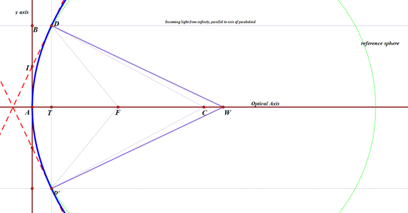
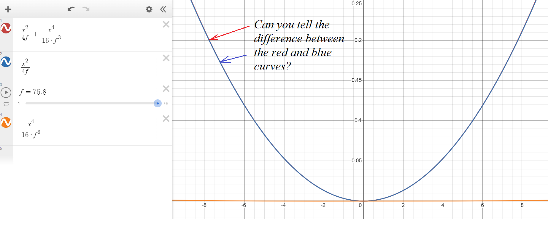
I claim that such a 3-dimensional paraboloid, like the radio dish in the picture below, can be represented by the equation
where f represents the focal length. (For simplicity, I have put the vertex of the paraboloid at the origin, which I have called A. I have decided to make the x-axis (green, pointing to our right) be the optical and geometric axis of the mirror. The positive z-axis (also green) is pointed towards our lower left, and the y-axis (again, green) is the vertical one. The focal point is somewhere on the x-axis, near the detector; let’s pretend it’s at the red dot that I labeled as Focus.)
You may be wondering where that immediately previous formula came from. Here is an explanation:
Let us define a paraboloid as the set (or locus) of all points in 3-D space that are equidistant from a given plane and a given focal point, whose coordinates I will arbitrarily call (f, 0, 0). (When deciding on a mirror or radio dish or reflector on a searchlight, you can make the focal length anything you want.)
To make it simple, the plane in question will be on the opposite side of the origin; its equation is x = -f. We will pick some random point G anywhere on the surface of the parabolic dish antenna and call its coordinates (x, y, z). We will see what equation these conditions create. We then drop a perpendicular from G towards the plane with equation x = -f. Where this perpendicular hits the plane, we will call point H, whose coordinates are (-f, y, z). We need for distance GH (from the point to the plane) to equal distance from G to the Focus. Distance GH is easy: it’s just f + x. To find distance between G and Focus, I will use the 3-D distance formula:
Which, after substituting, becomes
To get rid of the radical sign, I will equate those two quantities, because FG = GH, omit the zeroes, and square both sides. I then get
Multiplying out both sides, we get
Canceling equal stuff on both sides, I get
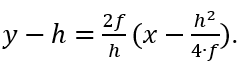
Adding 2fx to both sides, and dividing both sides by 4f, I then get
However, 3 dimensions is harder than 2 dimensions, and two dimensions will work just fine for right now. Let us just consider a slice through this paraboloid via the x-y plane, as you see below: a 2-dimensional cross-section of the 3-dimensional paraboloid, sliced through the vertex of the paraboloid, which you recall is at the origin. We can ignore the z values, because they will all be zero, so the equation for the blue parabola is
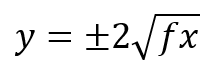
or, if you solve it for y, you get
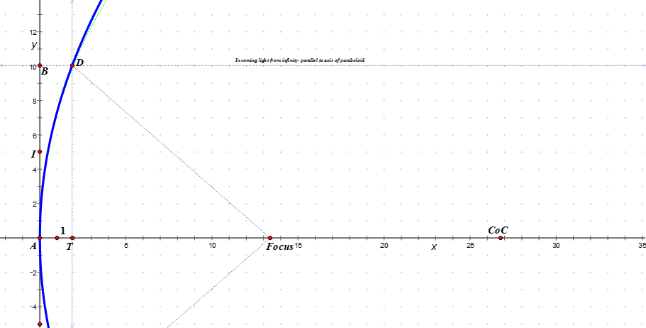
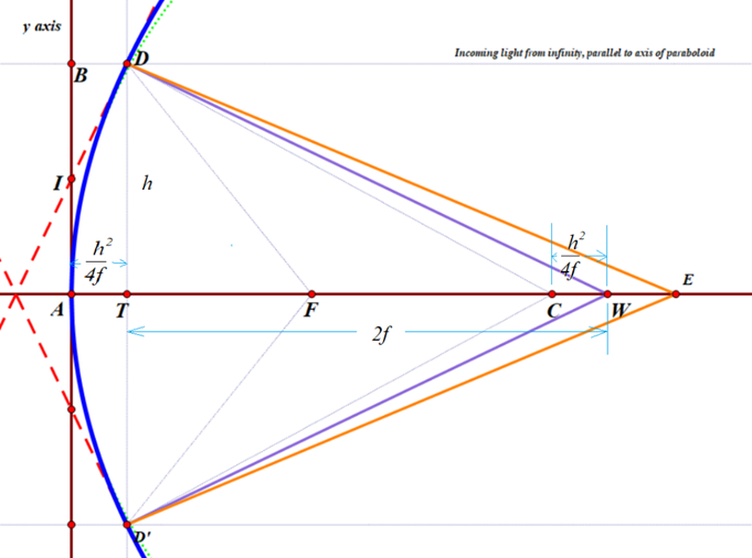
There is a circle with almost the same curvature as the paraboloid; its center, labeled CoC (for ‘Center of Curvature’) is exactly twice as far from the origin as the focal point. You can just barely see a green dotted curve representing that circle, towards the top of the diagram, just to the right of the blue paraboloid. center of the circle (and sphere). Its radius is 2f, which obviously depends on the location of the Focus.
D is a random point on that parabola, much like point G was earlier, and D’ being precisely on the opposite side of the optical axis. The great thing about parabolic mirrors is that every single incoming light ray coming into the paraboloid that is parallel to the axis will reflect towards the Focus, as we saw earlier. Or else, if you want to make a lamp or searchlight, and you place a light source at the focus, then all of the light that comes from it that bounces off of the mirror will be reflected out in a parallel beam that does not spread out.
In my diagram, you can see a very thin line, parallel to the x-axis, coming in from a distant star (meaning, effectively at infinity), bouncing off the parabola, and then hitting the Focus.
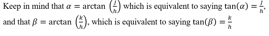
I also drew two red, dashed lines that are tangent to the paraboloid at point D and D’. I am calling the y-coordinate of point D as h (D has y-coordinate -h)and the x-coordinate of either one is
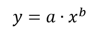
I used basic calculus to work out the slope of the red, dashed tangent line ID. (Quick reminder, if you forgot: in the very first part of most calculus classes, students learn that the derivative, or slope, of any function such as this:
is given by this:
So for the parabola with equation
the slope can be found for any value of x by plugging that value into the equation
Since
the exponent b is one-half. Therefore, the slope is going to be
which simplifies to
Now we need to plug in the x coordinate of point D, namely
we then get that the slope is
To find the equation of the tangent line, I used the point-slope formula y – y1=m(x – x1). ; plugging in my known values, I got the result
To find where this hits the y-axis, I substituted 0 for x, and got the result that the tangent line hits the y-axis at the point (0, h/2) — which I labeled as I — or one-half of the distance from the vertex (or origin) to the ‘height’ of the zone, or ring, being measured.
Line DW is constructed to be perpendicular to that tangent, so any beam of light coming from W that hits the parabola at point D will be reflected back upon itself. Perpendicular lines have slopes equal to the negative reciprocal of the other. Since the tangent has slope 2f/h, then line DW has slope -h/(2f).
Plugging in the known values into the point-slope formula, the equation for DW is therefore
Here, I am interested in the value of x when y = 0. Substituting, re-arranging, and solving for x, I get
Recall that point C is precisely 2f units from the origin, which means that the perpendicular line DW hits the x axis at a point that is the same distance from the center of curvature CoC as the point D is from the y-axis!
Or, in other words, CW = AT = DE. This means: if you are testing a parabolic mirror with a moving light source at point W, then a beam of light from W that is aimed at point D on the paraboloid will come right back to W, and the longitudinal readings of distance will follow the rule h2/(4f), where h is the radius of the zone, or ring, that you are measuring. Other locations on the mirror which do not lie in that ring will not have that property. This then is the derivation of the formula I was taught over 30 years ago by Jerry Schnall, and found in many books on telescope making – namely that for a moving light source, since R=2f,
where LA means ‘longitudinal aberration and the capital R is the radius of curvature of the mirror, or twice the focal length. So that’s exactly the same as what I computed.
HOWEVER, this formula [ LA=h^2/(2R) ] does not work at all if your light source is fixed at point C, the center of curvature of the green, reference sphere. In the old days, before the invention of LEDs, the light sources were fairly large and rather hot, so it was easier to make them stationary, and the user would move the knife-edge back and forth, but not the light source. The formula I was given for this arrangement by my mentor Jerry Schnall, and which is also given in numerous sources on telescope making was this:
that is, exactly twice as much as for a moving light source. I discovered to my surprise that this is not correct, but it took me a while to figure this out. I originally wrote the following:
But now I can confirm this, thanks in part to two of my very mathematically inclined 8th grade geometry students. Here goes, as corrected:
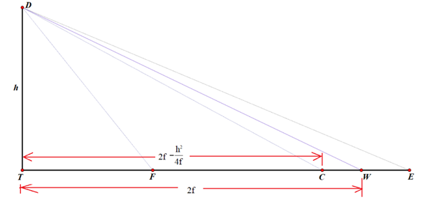
If one is using a fixed light source located at the center of curvature C, and a moving knife-edge, located at point E, the the rays of light that hit the same point D will NOT bounce straight back, because they don’t hit the tangent line at precisely 90 degrees. Instead, the angle of incidence CDW will equal the angle of reflection, namely WDE. I used Geometer’s sketchpad to construct line DE by asking the software to reflect line CD over the line DW.
However, calculating an algebraic expression for the x-coordinate of point E was surprisingly complicated. See if you can follow along!
To find the x-coordinate of E, I will employ the tangent of angle TDE.
To make the computations easier, I will draw a couple of simplified diagrams that keep the essentials.
I also tried other approaches, and also got answers that made no sense. It looks like the formula in the 1902 article is correct, but I have not been able to confirm it.
I suspect I made a very stupid and obvious algebra mistake that anybody who has made it through pre-calculus can easily find and point out to me, but I have had no luck in finding it so far. I would love for someone did to point it out to me.
A decade or so ago, I bought a brand-new Personal Solar Telescope from Hands On Optics. It was great! Not only could you see sunspots safely, but you could also make out prominences around the circumference of the sun, and if sky conditions were OK, you could make out plages, striations, and all sorts of other features on the Sun’s surface. If you were patient, you could tune the filters so that with the Doppler effect and the fact that many of the filaments and prominences are moving very quickly, you could make them appear and disappear as you changed the H-alpha frequency ever so slightly to one end of the spectrum to the other.
However, as the years went on, the Sun’s image got harder and harder to see. Finally I couldn’t see anything at all. And the Sun got quiet, so my PST just sat in its case, unused, for over a year. I was hoping it wasn’t my eyes!
I later found some information at Starry Nights on fixing the problem: one of the several filters (a ‘blocking’ or ‘ITF’ filter) not far in front of the eyepiece tends to get oxidized, and hence, opaque. I ordered a replacement from Meier at about $80, but was frankly rather apprehensive about figuring out how to do the actual deed. (Unfortunately they are now out of stock: https://maierphotonics.com/656bandpassfilter-1.aspx )
I finally found some threads on Starry Nights that explained more clearly what one was supposed to do ( https://www.cloudynights.com/topic/530890-newbie-trouble-with-coronado-pst/page-4 ) and with a pair of taped-up channel lock pliers and an old 3/4″ chisel that I ground down so that it would turn the threads on the retaining ring, I was able to remove the old filter and put in the new one. Here is a photo of the old filter (to the right, yellowish – blue) and the new one, which is so reflective you can see my red-and-blue cell phone with a fuzzy shiny Apple logo in the middle.
This afternoon, since for a change it wasn’t raining, I got to take it out and use it.